Discretización de la característica

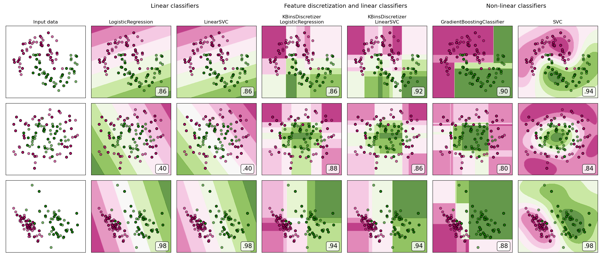
Demostración de la discretización de características en conjuntos de datos sintéticos de clasificación. La discretización de rasgos descompone cada rasgo en un conjunto de bines, en este caso distribuidos equitativamente en anchura. A continuación, los valores discretos se codifican en un solo paso y se entregan a un clasificador lineal. Este preprocesamiento permite un comportamiento no lineal aunque el clasificador sea lineal.

En este ejemplo, las dos primeras filas representan conjuntos de datos lineales no separables (lunas y círculos concentrados) mientras que la tercera es aproximadamente separable linealmente. En los dos conjuntos de datos lineales no separables, la discretización aumenta en gran medida el rendimiento de los clasificadores lineales. En el conjunto de datos lineales separables, la discretización de las características disminuye el rendimiento de los clasificadores lineales.

Este ejemplo debería tomarse con un grano de sal, ya que la intuición transmitida no necesariamente se transfiere a los conjuntos de datos reales. Particularmente en espacios de alta dimensión, los datos pueden separarse linealmente. Además, el uso de la discretización de características y la codificación de una sola en caliente aumenta el número de características, lo que fácilmente conduce a un exceso de ajuste cuando el número de muestras es pequeño.

Las gráficas muestran puntos de entrenamiento en colores sólidos y puntos de prueba semitransparentes.

Out:

dataset 0
---------
LogisticRegression: 0.86
LinearSVC: 0.86
KBinsDiscretizer + LogisticRegression: 0.86
KBinsDiscretizer + LinearSVC: 0.92
GradientBoostingClassifier: 0.90
SVC: 0.94

dataset 1
---------
LogisticRegression: 0.40
LinearSVC: 0.40
KBinsDiscretizer + LogisticRegression: 0.88
KBinsDiscretizer + LinearSVC: 0.86
GradientBoostingClassifier: 0.80
SVC: 0.84

dataset 2
---------
LogisticRegression: 0.98
LinearSVC: 0.98
KBinsDiscretizer + LogisticRegression: 0.94
KBinsDiscretizer + LinearSVC: 0.94
GradientBoostingClassifier: 0.88
SVC: 0.98

# Code source: Tom Dupré la Tour
# Adapted from plot_classifier_comparison by Gaël Varoquaux and Andreas Müller
#
# License: BSD 3 clause

import numpy as np
import matplotlib.pyplot as plt
from matplotlib.colors import ListedColormap
from sklearn.model_selection import train_test_split
from sklearn.preprocessing import StandardScaler
from sklearn.datasets import make_moons, make_circles, make_classification
from sklearn.linear_model import LogisticRegression
from sklearn.model_selection import GridSearchCV
from sklearn.pipeline import make_pipeline
from sklearn.preprocessing import KBinsDiscretizer
from sklearn.svm import SVC, LinearSVC
from sklearn.ensemble import GradientBoostingClassifier
from sklearn.utils._testing import ignore_warnings
from sklearn.exceptions import ConvergenceWarning

print(__doc__)

h = .02  # step size in the mesh


def get_name(estimator):
    name = estimator.__class__.__name__
    if name == 'Pipeline':
        name = [get_name(est[1]) for est in estimator.steps]
        name = ' + '.join(name)
    return name


# list of (estimator, param_grid), where param_grid is used in GridSearchCV
classifiers = [
    (LogisticRegression(random_state=0), {
        'C': np.logspace(-2, 7, 10)
    }),
    (LinearSVC(random_state=0), {
        'C': np.logspace(-2, 7, 10)
    }),
    (make_pipeline(
        KBinsDiscretizer(encode='onehot'),
        LogisticRegression(random_state=0)), {
            'kbinsdiscretizer__n_bins': np.arange(2, 10),
            'logisticregression__C': np.logspace(-2, 7, 10),
        }),
    (make_pipeline(
        KBinsDiscretizer(encode='onehot'), LinearSVC(random_state=0)), {
            'kbinsdiscretizer__n_bins': np.arange(2, 10),
            'linearsvc__C': np.logspace(-2, 7, 10),
        }),
    (GradientBoostingClassifier(n_estimators=50, random_state=0), {
        'learning_rate': np.logspace(-4, 0, 10)
    }),
    (SVC(random_state=0), {
        'C': np.logspace(-2, 7, 10)
    }),
]

names = [get_name(e) for e, g in classifiers]

n_samples = 100
datasets = [
    make_moons(n_samples=n_samples, noise=0.2, random_state=0),
    make_circles(n_samples=n_samples, noise=0.2, factor=0.5, random_state=1),
    make_classification(n_samples=n_samples, n_features=2, n_redundant=0,
                        n_informative=2, random_state=2,
                        n_clusters_per_class=1)
]

fig, axes = plt.subplots(nrows=len(datasets), ncols=len(classifiers) + 1,
                         figsize=(21, 9))

cm = plt.cm.PiYG
cm_bright = ListedColormap(['#b30065', '#178000'])

# iterate over datasets
for ds_cnt, (X, y) in enumerate(datasets):
    print('\ndataset %d\n---------' % ds_cnt)

    # preprocess dataset, split into training and test part
    X = StandardScaler().fit_transform(X)
    X_train, X_test, y_train, y_test = train_test_split(
        X, y, test_size=.5, random_state=42)

    # create the grid for background colors
    x_min, x_max = X[:, 0].min() - .5, X[:, 0].max() + .5
    y_min, y_max = X[:, 1].min() - .5, X[:, 1].max() + .5
    xx, yy = np.meshgrid(
        np.arange(x_min, x_max, h), np.arange(y_min, y_max, h))

    # plot the dataset first
    ax = axes[ds_cnt, 0]
    if ds_cnt == 0:
        ax.set_title("Input data")
    # plot the training points
    ax.scatter(X_train[:, 0], X_train[:, 1], c=y_train, cmap=cm_bright,
               edgecolors='k')
    # and testing points
    ax.scatter(X_test[:, 0], X_test[:, 1], c=y_test, cmap=cm_bright, alpha=0.6,
               edgecolors='k')
    ax.set_xlim(xx.min(), xx.max())
    ax.set_ylim(yy.min(), yy.max())
    ax.set_xticks(())
    ax.set_yticks(())

    # iterate over classifiers
    for est_idx, (name, (estimator, param_grid)) in \
            enumerate(zip(names, classifiers)):
        ax = axes[ds_cnt, est_idx + 1]

        clf = GridSearchCV(estimator=estimator, param_grid=param_grid)
        with ignore_warnings(category=ConvergenceWarning):
            clf.fit(X_train, y_train)
        score = clf.score(X_test, y_test)
        print('%s: %.2f' % (name, score))

        # plot the decision boundary. For that, we will assign a color to each
        # point in the mesh [x_min, x_max]*[y_min, y_max].
        if hasattr(clf, "decision_function"):
            Z = clf.decision_function(np.c_[xx.ravel(), yy.ravel()])
        else:
            Z = clf.predict_proba(np.c_[xx.ravel(), yy.ravel()])[:, 1]

        # put the result into a color plot
        Z = Z.reshape(xx.shape)
        ax.contourf(xx, yy, Z, cmap=cm, alpha=.8)

        # plot the training points
        ax.scatter(X_train[:, 0], X_train[:, 1], c=y_train, cmap=cm_bright,
                   edgecolors='k')
        # and testing points
        ax.scatter(X_test[:, 0], X_test[:, 1], c=y_test, cmap=cm_bright,
                   edgecolors='k', alpha=0.6)
        ax.set_xlim(xx.min(), xx.max())
        ax.set_ylim(yy.min(), yy.max())
        ax.set_xticks(())
        ax.set_yticks(())

        if ds_cnt == 0:
            ax.set_title(name.replace(' + ', '\n'))
        ax.text(0.95, 0.06, ('%.2f' % score).lstrip('0'), size=15,
                bbox=dict(boxstyle='round', alpha=0.8, facecolor='white'),
                transform=ax.transAxes, horizontalalignment='right')


plt.tight_layout()

# Add suptitles above the figure
plt.subplots_adjust(top=0.90)
suptitles = [
    'Linear classifiers',
    'Feature discretization and linear classifiers',
    'Non-linear classifiers',
]
for i, suptitle in zip([1, 3, 5], suptitles):
    ax = axes[0, i]
    ax.text(1.05, 1.25, suptitle, transform=ax.transAxes,
            horizontalalignment='center', size='x-large')
plt.show()