Regresión de procesos Gaussianos: ejemplo introductorio básico

Un ejemplo simple de regresión unidimensional calculado de dos maneras diferentes:

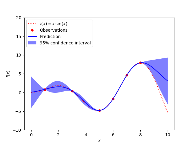
1. Un caso libre de ruido

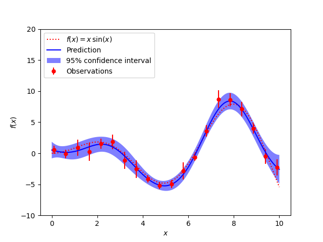
2. Un caso ruidoso con un nivel de ruido conocido por punto de datos

En ambos casos, los parámetros del núcleo se calculan utilizando el principio de verosimilitud máxima.

Las cifras ilustran la propiedad interpolante del modelo del Proceso Gaussiano así como su naturaleza probabilística en forma de un intervalo de confianza del 95% sin sentido.

Ten en cuenta que el parámetro alpha se aplica como una regularización Tikhonov de la covarianza asumida entre los puntos de entrenamiento.

• 
• 

print(__doc__)

# Author: Vincent Dubourg <vincent.dubourg@gmail.com>
#         Jake Vanderplas <vanderplas@astro.washington.edu>
#         Jan Hendrik Metzen <jhm@informatik.uni-bremen.de>s
# License: BSD 3 clause

import numpy as np
from matplotlib import pyplot as plt

from sklearn.gaussian_process import GaussianProcessRegressor
from sklearn.gaussian_process.kernels import RBF, ConstantKernel as C

np.random.seed(1)


def f(x):
    """The function to predict."""
    return x * np.sin(x)

# ----------------------------------------------------------------------
#  First the noiseless case
X = np.atleast_2d([1., 3., 5., 6., 7., 8.]).T

# Observations
y = f(X).ravel()

# Mesh the input space for evaluations of the real function, the prediction and
# its MSE
x = np.atleast_2d(np.linspace(0, 10, 1000)).T

# Instantiate a Gaussian Process model
kernel = C(1.0, (1e-3, 1e3)) * RBF(10, (1e-2, 1e2))
gp = GaussianProcessRegressor(kernel=kernel, n_restarts_optimizer=9)

# Fit to data using Maximum Likelihood Estimation of the parameters
gp.fit(X, y)

# Make the prediction on the meshed x-axis (ask for MSE as well)
y_pred, sigma = gp.predict(x, return_std=True)

# Plot the function, the prediction and the 95% confidence interval based on
# the MSE
plt.figure()
plt.plot(x, f(x), 'r:', label=r'$f(x) = x\,\sin(x)$')
plt.plot(X, y, 'r.', markersize=10, label='Observations')
plt.plot(x, y_pred, 'b-', label='Prediction')
plt.fill(np.concatenate([x, x[::-1]]),
         np.concatenate([y_pred - 1.9600 * sigma,
                        (y_pred + 1.9600 * sigma)[::-1]]),
         alpha=.5, fc='b', ec='None', label='95% confidence interval')
plt.xlabel('$x$')
plt.ylabel('$f(x)$')
plt.ylim(-10, 20)
plt.legend(loc='upper left')

# ----------------------------------------------------------------------
# now the noisy case
X = np.linspace(0.1, 9.9, 20)
X = np.atleast_2d(X).T

# Observations and noise
y = f(X).ravel()
dy = 0.5 + 1.0 * np.random.random(y.shape)
noise = np.random.normal(0, dy)
y += noise

# Instantiate a Gaussian Process model
gp = GaussianProcessRegressor(kernel=kernel, alpha=dy ** 2,
                              n_restarts_optimizer=10)

# Fit to data using Maximum Likelihood Estimation of the parameters
gp.fit(X, y)

# Make the prediction on the meshed x-axis (ask for MSE as well)
y_pred, sigma = gp.predict(x, return_std=True)

# Plot the function, the prediction and the 95% confidence interval based on
# the MSE
plt.figure()
plt.plot(x, f(x), 'r:', label=r'$f(x) = x\,\sin(x)$')
plt.errorbar(X.ravel(), y, dy, fmt='r.', markersize=10, label='Observations')
plt.plot(x, y_pred, 'b-', label='Prediction')
plt.fill(np.concatenate([x, x[::-1]]),
         np.concatenate([y_pred - 1.9600 * sigma,
                        (y_pred + 1.9600 * sigma)[::-1]]),
         alpha=.5, fc='b', ec='None', label='95% confidence interval')
plt.xlabel('$x$')
plt.ylabel('$f(x)$')
plt.ylim(-10, 20)
plt.legend(loc='upper left')

plt.show()