Regresión del proceso gaussiano (GPR) con estimación a nivel de ruido

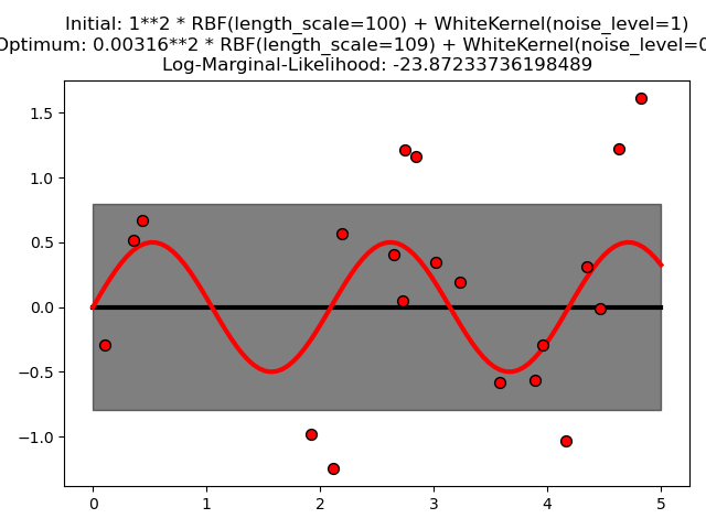
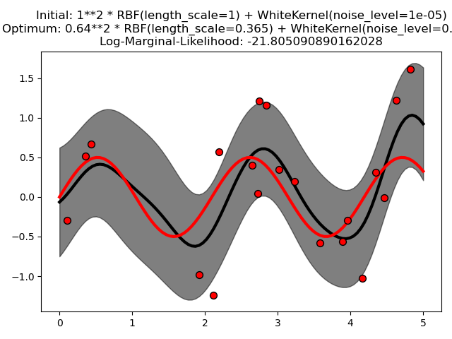
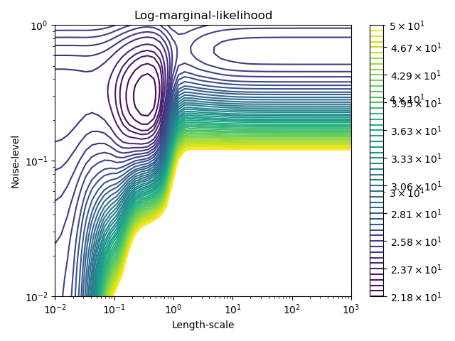
Este ejemplo ilustra que la GPR con un núcleo de suma que incluye un núcleo blanco puede estimar el nivel de ruido de los datos. Una ilustración del paisaje de la verosimilitud marginal logarítmica (LML) muestra que existen dos máximos locales de LML. El primero corresponde a un modelo con un alto nivel de ruido y una gran escala de longitud, que explica todas las variaciones de los datos por el ruido. El segundo tiene un nivel de ruido menor y una escala de longitud más corta, que explica la mayor parte de la variación por la relación funcional sin ruido. El segundo modelo tiene una mayor verosimilitud; sin embargo, dependiendo del valor inicial de los hiperparámetros, la optimización basada en el gradiente también podría converger a la solución de alto ruido. Por lo tanto, es importante repetir la optimización varias veces para diferentes inicializaciones.

• 
• 
• 

Out:

/home/mapologo/miniconda3/envs/sklearn/lib/python3.9/site-packages/scikit_learn-0.24.1-py3.9-linux-x86_64.egg/sklearn/gaussian_process/kernels.py:402: ConvergenceWarning: The optimal value found for dimension 0 of parameter k1__k1__constant_value is close to the specified lower bound 1e-05. Decreasing the bound and calling fit again may find a better value.
  warnings.warn("The optimal value found for "

print(__doc__)

# Authors: Jan Hendrik Metzen <jhm@informatik.uni-bremen.de>
#
# License: BSD 3 clause

import numpy as np

from matplotlib import pyplot as plt
from matplotlib.colors import LogNorm

from sklearn.gaussian_process import GaussianProcessRegressor
from sklearn.gaussian_process.kernels import RBF, WhiteKernel


rng = np.random.RandomState(0)
X = rng.uniform(0, 5, 20)[:, np.newaxis]
y = 0.5 * np.sin(3 * X[:, 0]) + rng.normal(0, 0.5, X.shape[0])

# First run
plt.figure()
kernel = 1.0 * RBF(length_scale=100.0, length_scale_bounds=(1e-2, 1e3)) \
    + WhiteKernel(noise_level=1, noise_level_bounds=(1e-10, 1e+1))
gp = GaussianProcessRegressor(kernel=kernel,
                              alpha=0.0).fit(X, y)
X_ = np.linspace(0, 5, 100)
y_mean, y_cov = gp.predict(X_[:, np.newaxis], return_cov=True)
plt.plot(X_, y_mean, 'k', lw=3, zorder=9)
plt.fill_between(X_, y_mean - np.sqrt(np.diag(y_cov)),
                 y_mean + np.sqrt(np.diag(y_cov)),
                 alpha=0.5, color='k')
plt.plot(X_, 0.5*np.sin(3*X_), 'r', lw=3, zorder=9)
plt.scatter(X[:, 0], y, c='r', s=50, zorder=10, edgecolors=(0, 0, 0))
plt.title("Initial: %s\nOptimum: %s\nLog-Marginal-Likelihood: %s"
          % (kernel, gp.kernel_,
             gp.log_marginal_likelihood(gp.kernel_.theta)))
plt.tight_layout()

# Second run
plt.figure()
kernel = 1.0 * RBF(length_scale=1.0, length_scale_bounds=(1e-2, 1e3)) \
    + WhiteKernel(noise_level=1e-5, noise_level_bounds=(1e-10, 1e+1))
gp = GaussianProcessRegressor(kernel=kernel,
                              alpha=0.0).fit(X, y)
X_ = np.linspace(0, 5, 100)
y_mean, y_cov = gp.predict(X_[:, np.newaxis], return_cov=True)
plt.plot(X_, y_mean, 'k', lw=3, zorder=9)
plt.fill_between(X_, y_mean - np.sqrt(np.diag(y_cov)),
                 y_mean + np.sqrt(np.diag(y_cov)),
                 alpha=0.5, color='k')
plt.plot(X_, 0.5*np.sin(3*X_), 'r', lw=3, zorder=9)
plt.scatter(X[:, 0], y, c='r', s=50, zorder=10, edgecolors=(0, 0, 0))
plt.title("Initial: %s\nOptimum: %s\nLog-Marginal-Likelihood: %s"
          % (kernel, gp.kernel_,
             gp.log_marginal_likelihood(gp.kernel_.theta)))
plt.tight_layout()

# Plot LML landscape
plt.figure()
theta0 = np.logspace(-2, 3, 49)
theta1 = np.logspace(-2, 0, 50)
Theta0, Theta1 = np.meshgrid(theta0, theta1)
LML = [[gp.log_marginal_likelihood(np.log([0.36, Theta0[i, j], Theta1[i, j]]))
        for i in range(Theta0.shape[0])] for j in range(Theta0.shape[1])]
LML = np.array(LML).T

vmin, vmax = (-LML).min(), (-LML).max()
vmax = 50
level = np.around(np.logspace(np.log10(vmin), np.log10(vmax), 50), decimals=1)
plt.contour(Theta0, Theta1, -LML,
            levels=level, norm=LogNorm(vmin=vmin, vmax=vmax))
plt.colorbar()
plt.xscale("log")
plt.yscale("log")
plt.xlabel("Length-scale")
plt.ylabel("Noise-level")
plt.title("Log-marginal-likelihood")
plt.tight_layout()

plt.show()