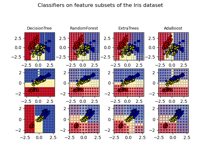
Graficar las superficies de decisión de los ensembles de árboles en el conjunto de datos iris

Graficar las superficies de decisión de los bosques de árboles aleatorios entrenados en pares de características del conjunto de datos iris.

Este gráfico compara las superficies de decisión aprendidas por un clasificador de árbol de decisión (primera columna), por un clasificador de bosque aleatorio (segunda columna), por un clasificador de árboles extra (tercera columna) y por un clasificador AdaBoost (cuarta columna).

En la primera fila, los clasificadores se construyen utilizando sólo las características de la anchura y la longitud del sépalo, en la segunda fila utilizando sólo la longitud del pétalo y la longitud del sépalo, y en la tercera fila utilizando sólo la anchura del pétalo y la longitud del pétalo.

En orden descendente de calidad, cuando se entrena (fuera de este ejemplo) en las 4 características utilizando 30 estimadores y se puntúa utilizando una validación cruzada de 10 veces, vemos:

ExtraTreesClassifier()  # 0.95 score
RandomForestClassifier()  # 0.94 score
AdaBoost(DecisionTree(max_depth=3))  # 0.94 score
DecisionTree(max_depth=None)  # 0.94 score

El aumento de max_depth para AdaBoost reduce la desviación estándar de las puntuaciones (pero la puntuación media no mejora).

Ver la salida de la consola para más detalles sobre cada modelo.

En este ejemplo se podría intentar:

1. variar la max_depth para el DecisionTreeClassifier y AdaBoostClassifier, quizás probar max_depth=3 para el DecisionTreeClassifier o max_depth=None por AdaBoostClassifier

2. variar n_estimators

Cabe destacar que RandomForests y ExtraTrees pueden ajustarse en paralelo en muchos núcleos, ya que cada árbol se construye independientemente de los demás. Las muestras de AdaBoost se construyen de forma secuencial y, por tanto, no utilizan varios núcleos.

Out:

DecisionTree with features [0, 1] has a score of 0.9266666666666666
RandomForest with 30 estimators with features [0, 1] has a score of 0.9266666666666666
ExtraTrees with 30 estimators with features [0, 1] has a score of 0.9266666666666666
AdaBoost with 30 estimators with features [0, 1] has a score of 0.8533333333333334
DecisionTree with features [0, 2] has a score of 0.9933333333333333
RandomForest with 30 estimators with features [0, 2] has a score of 0.9933333333333333
ExtraTrees with 30 estimators with features [0, 2] has a score of 0.9933333333333333
AdaBoost with 30 estimators with features [0, 2] has a score of 0.9933333333333333
DecisionTree with features [2, 3] has a score of 0.9933333333333333
RandomForest with 30 estimators with features [2, 3] has a score of 0.9933333333333333
ExtraTrees with 30 estimators with features [2, 3] has a score of 0.9933333333333333
AdaBoost with 30 estimators with features [2, 3] has a score of 0.9933333333333333

print(__doc__)

import numpy as np
import matplotlib.pyplot as plt
from matplotlib.colors import ListedColormap

from sklearn.datasets import load_iris
from sklearn.ensemble import (RandomForestClassifier, ExtraTreesClassifier,
                              AdaBoostClassifier)
from sklearn.tree import DecisionTreeClassifier

# Parameters
n_classes = 3
n_estimators = 30
cmap = plt.cm.RdYlBu
plot_step = 0.02  # fine step width for decision surface contours
plot_step_coarser = 0.5  # step widths for coarse classifier guesses
RANDOM_SEED = 13  # fix the seed on each iteration

# Load data
iris = load_iris()

plot_idx = 1

models = [DecisionTreeClassifier(max_depth=None),
          RandomForestClassifier(n_estimators=n_estimators),
          ExtraTreesClassifier(n_estimators=n_estimators),
          AdaBoostClassifier(DecisionTreeClassifier(max_depth=3),
                             n_estimators=n_estimators)]

for pair in ([0, 1], [0, 2], [2, 3]):
    for model in models:
        # We only take the two corresponding features
        X = iris.data[:, pair]
        y = iris.target

        # Shuffle
        idx = np.arange(X.shape[0])
        np.random.seed(RANDOM_SEED)
        np.random.shuffle(idx)
        X = X[idx]
        y = y[idx]

        # Standardize
        mean = X.mean(axis=0)
        std = X.std(axis=0)
        X = (X - mean) / std

        # Train
        model.fit(X, y)

        scores = model.score(X, y)
        # Create a title for each column and the console by using str() and
        # slicing away useless parts of the string
        model_title = str(type(model)).split(
            ".")[-1][:-2][:-len("Classifier")]

        model_details = model_title
        if hasattr(model, "estimators_"):
            model_details += " with {} estimators".format(
                len(model.estimators_))
        print(model_details + " with features", pair,
              "has a score of", scores)

        plt.subplot(3, 4, plot_idx)
        if plot_idx <= len(models):
            # Add a title at the top of each column
            plt.title(model_title, fontsize=9)

        # Now plot the decision boundary using a fine mesh as input to a
        # filled contour plot
        x_min, x_max = X[:, 0].min() - 1, X[:, 0].max() + 1
        y_min, y_max = X[:, 1].min() - 1, X[:, 1].max() + 1
        xx, yy = np.meshgrid(np.arange(x_min, x_max, plot_step),
                             np.arange(y_min, y_max, plot_step))

        # Plot either a single DecisionTreeClassifier or alpha blend the
        # decision surfaces of the ensemble of classifiers
        if isinstance(model, DecisionTreeClassifier):
            Z = model.predict(np.c_[xx.ravel(), yy.ravel()])
            Z = Z.reshape(xx.shape)
            cs = plt.contourf(xx, yy, Z, cmap=cmap)
        else:
            # Choose alpha blend level with respect to the number
            # of estimators
            # that are in use (noting that AdaBoost can use fewer estimators
            # than its maximum if it achieves a good enough fit early on)
            estimator_alpha = 1.0 / len(model.estimators_)
            for tree in model.estimators_:
                Z = tree.predict(np.c_[xx.ravel(), yy.ravel()])
                Z = Z.reshape(xx.shape)
                cs = plt.contourf(xx, yy, Z, alpha=estimator_alpha, cmap=cmap)

        # Build a coarser grid to plot a set of ensemble classifications
        # to show how these are different to what we see in the decision
        # surfaces. These points are regularly space and do not have a
        # black outline
        xx_coarser, yy_coarser = np.meshgrid(
            np.arange(x_min, x_max, plot_step_coarser),
            np.arange(y_min, y_max, plot_step_coarser))
        Z_points_coarser = model.predict(np.c_[xx_coarser.ravel(),
                                         yy_coarser.ravel()]
                                         ).reshape(xx_coarser.shape)
        cs_points = plt.scatter(xx_coarser, yy_coarser, s=15,
                                c=Z_points_coarser, cmap=cmap,
                                edgecolors="none")

        # Plot the training points, these are clustered together and have a
        # black outline
        plt.scatter(X[:, 0], X[:, 1], c=y,
                    cmap=ListedColormap(['r', 'y', 'b']),
                    edgecolor='k', s=20)
        plot_idx += 1  # move on to the next plot in sequence

plt.suptitle("Classifiers on feature subsets of the Iris dataset", fontsize=12)
plt.axis("tight")
plt.tight_layout(h_pad=0.2, w_pad=0.2, pad=2.5)
plt.show()