Estimación de la Densidad del Núcleo de las Distribuciones de las Especies

Muestra un ejemplo de consulta basada en vecinos (en particular, una estimación de la densidad núcleo) sobre datos geoespaciales, utilizando un Árbol de Bolas construido sobre la métrica de distancia de Haversine, es decir, distancias sobre puntos en latitud/longitud. El conjunto de datos es proporcionado por Phillips et. al. (2006). Si está disponible, el ejemplo utiliza basemap para trazar las líneas de costa y las fronteras nacionales de Sudamérica.

Este ejemplo no realiza ningún aprendizaje sobre los datos (ver Modelización de la distribución de las especies para un ejemplo de clasificación basado en los atributos de este conjunto de datos). Simplemente muestra la estimación de la densidad núcleo de los puntos de datos observados en coordenadas geoespaciales.

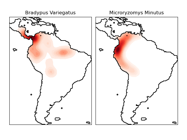
Las dos especies son:

• «Bradypus variegatus» , el perezoso de garganta marrón.

• «Microryzomys minutus» , también conocido como la Pequeña Rata del Arroz del Bosque, un roedor que vive en Perú, Colombia, Ecuador y Venezuela.

Referencias

• «Maximum entropy modeling of species geographic distributions» S. J. Phillips, R. P. Anderson, R. E. Schapire - Ecological Modelling, 190:231-259, 2006.

Out:

- computing KDE in spherical coordinates
- plot coastlines from coverage
- computing KDE in spherical coordinates
- plot coastlines from coverage

# Author: Jake Vanderplas <jakevdp@cs.washington.edu>
#
# License: BSD 3 clause

import numpy as np
import matplotlib.pyplot as plt
from sklearn.datasets import fetch_species_distributions
from sklearn.neighbors import KernelDensity

# if basemap is available, we'll use it.
# otherwise, we'll improvise later...
try:
    from mpl_toolkits.basemap import Basemap
    basemap = True
except ImportError:
    basemap = False


def construct_grids(batch):
    """Construct the map grid from the batch object

    Parameters
    ----------
    batch : Batch object
        The object returned by :func:`fetch_species_distributions`

    Returns
    -------
    (xgrid, ygrid) : 1-D arrays
        The grid corresponding to the values in batch.coverages
    """
    # x,y coordinates for corner cells
    xmin = batch.x_left_lower_corner + batch.grid_size
    xmax = xmin + (batch.Nx * batch.grid_size)
    ymin = batch.y_left_lower_corner + batch.grid_size
    ymax = ymin + (batch.Ny * batch.grid_size)

    # x coordinates of the grid cells
    xgrid = np.arange(xmin, xmax, batch.grid_size)
    # y coordinates of the grid cells
    ygrid = np.arange(ymin, ymax, batch.grid_size)

    return (xgrid, ygrid)


# Get matrices/arrays of species IDs and locations
data = fetch_species_distributions()
species_names = ['Bradypus Variegatus', 'Microryzomys Minutus']

Xtrain = np.vstack([data['train']['dd lat'],
                    data['train']['dd long']]).T
ytrain = np.array([d.decode('ascii').startswith('micro')
                  for d in data['train']['species']], dtype='int')
Xtrain *= np.pi / 180.  # Convert lat/long to radians

# Set up the data grid for the contour plot
xgrid, ygrid = construct_grids(data)
X, Y = np.meshgrid(xgrid[::5], ygrid[::5][::-1])
land_reference = data.coverages[6][::5, ::5]
land_mask = (land_reference > -9999).ravel()

xy = np.vstack([Y.ravel(), X.ravel()]).T
xy = xy[land_mask]
xy *= np.pi / 180.

# Plot map of South America with distributions of each species
fig = plt.figure()
fig.subplots_adjust(left=0.05, right=0.95, wspace=0.05)

for i in range(2):
    plt.subplot(1, 2, i + 1)

    # construct a kernel density estimate of the distribution
    print(" - computing KDE in spherical coordinates")
    kde = KernelDensity(bandwidth=0.04, metric='haversine',
                        kernel='gaussian', algorithm='ball_tree')
    kde.fit(Xtrain[ytrain == i])

    # evaluate only on the land: -9999 indicates ocean
    Z = np.full(land_mask.shape[0], -9999, dtype='int')
    Z[land_mask] = np.exp(kde.score_samples(xy))
    Z = Z.reshape(X.shape)

    # plot contours of the density
    levels = np.linspace(0, Z.max(), 25)
    plt.contourf(X, Y, Z, levels=levels, cmap=plt.cm.Reds)

    if basemap:
        print(" - plot coastlines using basemap")
        m = Basemap(projection='cyl', llcrnrlat=Y.min(),
                    urcrnrlat=Y.max(), llcrnrlon=X.min(),
                    urcrnrlon=X.max(), resolution='c')
        m.drawcoastlines()
        m.drawcountries()
    else:
        print(" - plot coastlines from coverage")
        plt.contour(X, Y, land_reference,
                    levels=[-9998], colors="k",
                    linestyles="solid")
        plt.xticks([])
        plt.yticks([])

    plt.title(species_names[i])

plt.show()