Agrupamiento jerárquico: sala estructurada o no estructurada

El ejemplo construye un conjunto de datos de rollos suizos y ejecuta el agrupamiento jerárquico en su posición.

Para más información, consulta Análisis de conglomerados jerárquicos.

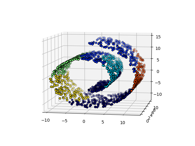
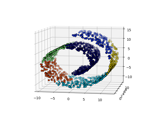
En un primer paso, el agrupamiento jerárquico se realiza sin restricciones de conectividad en la estructura y se basa únicamente en la distancia, mientras que en un segundo paso el agrupamiento se restringe al grafo k-vecinos más cercanos: es un agrupamiento jerárquico con estructura a priori.

Algunos de los conglomerados aprendidos sin restricciones de conectividad no respetan la estructura del rollo suizo y se extienden por diferentes pliegues de los colectores. Por el contrario, cuando se oponen las restricciones de conectividad, los conglomerados forman una bonita parcelación del rollo suizo.

• 
• 

Out:

Compute unstructured hierarchical clustering...
Elapsed time: 0.05s
Number of points: 1500
Compute structured hierarchical clustering...
Elapsed time: 0.18s
Number of points: 1500

# Authors : Vincent Michel, 2010
#           Alexandre Gramfort, 2010
#           Gael Varoquaux, 2010
# License: BSD 3 clause

print(__doc__)

import time as time
import numpy as np
import matplotlib.pyplot as plt
import mpl_toolkits.mplot3d.axes3d as p3
from sklearn.cluster import AgglomerativeClustering
from sklearn.datasets import make_swiss_roll

# #############################################################################
# Generate data (swiss roll dataset)
n_samples = 1500
noise = 0.05
X, _ = make_swiss_roll(n_samples, noise=noise)
# Make it thinner
X[:, 1] *= .5

# #############################################################################
# Compute clustering
print("Compute unstructured hierarchical clustering...")
st = time.time()
ward = AgglomerativeClustering(n_clusters=6, linkage='ward').fit(X)
elapsed_time = time.time() - st
label = ward.labels_
print("Elapsed time: %.2fs" % elapsed_time)
print("Number of points: %i" % label.size)

# #############################################################################
# Plot result
fig = plt.figure()
ax = p3.Axes3D(fig)
ax.view_init(7, -80)
for l in np.unique(label):
    ax.scatter(X[label == l, 0], X[label == l, 1], X[label == l, 2],
               color=plt.cm.jet(float(l) / np.max(label + 1)),
               s=20, edgecolor='k')
plt.title('Without connectivity constraints (time %.2fs)' % elapsed_time)


# #############################################################################
# Define the structure A of the data. Here a 10 nearest neighbors
from sklearn.neighbors import kneighbors_graph
connectivity = kneighbors_graph(X, n_neighbors=10, include_self=False)

# #############################################################################
# Compute clustering
print("Compute structured hierarchical clustering...")
st = time.time()
ward = AgglomerativeClustering(n_clusters=6, connectivity=connectivity,
                               linkage='ward').fit(X)
elapsed_time = time.time() - st
label = ward.labels_
print("Elapsed time: %.2fs" % elapsed_time)
print("Number of points: %i" % label.size)

# #############################################################################
# Plot result
fig = plt.figure()
ax = p3.Axes3D(fig)
ax.view_init(7, -80)
for l in np.unique(label):
    ax.scatter(X[label == l, 0], X[label == l, 1], X[label == l, 2],
               color=plt.cm.jet(float(l) / np.max(label + 1)),
               s=20, edgecolor='k')
plt.title('With connectivity constraints (time %.2fs)' % elapsed_time)

plt.show()