Segmentación de la imagen de las monedas griegas en regiones

Este ejemplo utiliza Análisis espectral de conglomerados en un grafo creado a partir de la diferencia entre vóxeles de una imagen para dividir esta imagen en múltiples regiones parcialmente homogéneas.

Este procedimiento (agrupamiento espectral sobre una imagen) es una solución aproximada eficiente para encontrar cortes de grafos normalizados.

Hay dos opciones para asignar etiquetas:

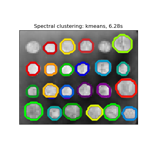
• con el agrupamiento espectral “kmeans” agrupará las muestras en el espacio de incrustación utilizando un algoritmo kmedias

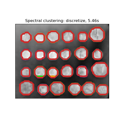
• mientras que “discrete” buscará iterativamente el espacio de partición más cercano al espacio de incrustación.

print(__doc__)

# Author: Gael Varoquaux <gael.varoquaux@normalesup.org>, Brian Cheung
# License: BSD 3 clause

import time

import numpy as np
from scipy.ndimage.filters import gaussian_filter
import matplotlib.pyplot as plt
import skimage
from skimage.data import coins
from skimage.transform import rescale

from sklearn.feature_extraction import image
from sklearn.cluster import spectral_clustering
from sklearn.utils.fixes import parse_version

# these were introduced in skimage-0.14
if parse_version(skimage.__version__) >= parse_version('0.14'):
    rescale_params = {'anti_aliasing': False, 'multichannel': False}
else:
    rescale_params = {}

# load the coins as a numpy array
orig_coins = coins()

# Resize it to 20% of the original size to speed up the processing
# Applying a Gaussian filter for smoothing prior to down-scaling
# reduces aliasing artifacts.
smoothened_coins = gaussian_filter(orig_coins, sigma=2)
rescaled_coins = rescale(smoothened_coins, 0.2, mode="reflect",
                         **rescale_params)

# Convert the image into a graph with the value of the gradient on the
# edges.
graph = image.img_to_graph(rescaled_coins)

# Take a decreasing function of the gradient: an exponential
# The smaller beta is, the more independent the segmentation is of the
# actual image. For beta=1, the segmentation is close to a voronoi
beta = 10
eps = 1e-6
graph.data = np.exp(-beta * graph.data / graph.data.std()) + eps

# Apply spectral clustering (this step goes much faster if you have pyamg
# installed)
N_REGIONS = 25

Visualizar las regiones resultantes

for assign_labels in ('kmeans', 'discretize'):
    t0 = time.time()
    labels = spectral_clustering(graph, n_clusters=N_REGIONS,
                                 assign_labels=assign_labels, random_state=42)
    t1 = time.time()
    labels = labels.reshape(rescaled_coins.shape)

    plt.figure(figsize=(5, 5))
    plt.imshow(rescaled_coins, cmap=plt.cm.gray)
    for l in range(N_REGIONS):
        plt.contour(labels == l,
                    colors=[plt.cm.nipy_spectral(l / float(N_REGIONS))])
    plt.xticks(())
    plt.yticks(())
    title = 'Spectral clustering: %s, %.2fs' % (assign_labels, (t1 - t0))
    print(title)
    plt.title(title)
plt.show()

• 
• 

Out:

Spectral clustering: kmeans, 6.28s
Spectral clustering: discretize, 5.46s