Agrupamiento por K-Medias

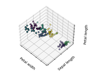
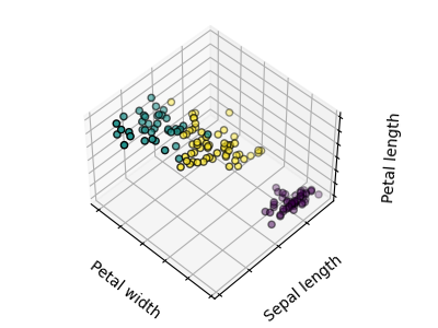
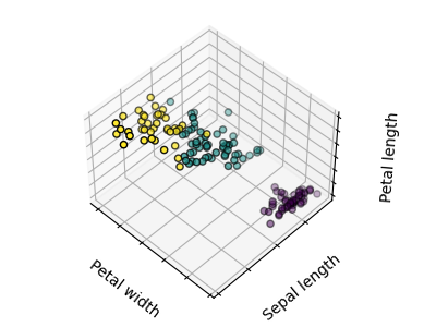
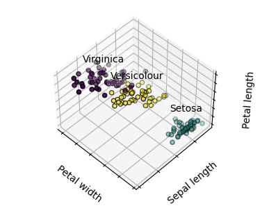
Los gráficos muestran, en primer lugar, lo que produciría un algoritmo K-medias utilizando tres conglomerados. A continuación se muestra cuál es el efecto de una mala inicialización en el proceso de clasificación: Al establecer n_init en sólo 1 (por defecto es 10), se reduce la cantidad de veces que el algoritmo se ejecutará con diferentes semillas de centroides. El siguiente gráfico muestra lo que se obtendría utilizando ocho conglomerados y, finalmente, la verdad fundamental.

• 
• 
• 
• 

print(__doc__)


# Code source: Gaël Varoquaux
# Modified for documentation by Jaques Grobler
# License: BSD 3 clause

import numpy as np
import matplotlib.pyplot as plt
# Though the following import is not directly being used, it is required
# for 3D projection to work
from mpl_toolkits.mplot3d import Axes3D

from sklearn.cluster import KMeans
from sklearn import datasets

np.random.seed(5)

iris = datasets.load_iris()
X = iris.data
y = iris.target

estimators = [('k_means_iris_8', KMeans(n_clusters=8)),
              ('k_means_iris_3', KMeans(n_clusters=3)),
              ('k_means_iris_bad_init', KMeans(n_clusters=3, n_init=1,
                                               init='random'))]

fignum = 1
titles = ['8 clusters', '3 clusters', '3 clusters, bad initialization']
for name, est in estimators:
    fig = plt.figure(fignum, figsize=(4, 3))
    ax = Axes3D(fig, rect=[0, 0, .95, 1], elev=48, azim=134)
    est.fit(X)
    labels = est.labels_

    ax.scatter(X[:, 3], X[:, 0], X[:, 2],
               c=labels.astype(float), edgecolor='k')

    ax.w_xaxis.set_ticklabels([])
    ax.w_yaxis.set_ticklabels([])
    ax.w_zaxis.set_ticklabels([])
    ax.set_xlabel('Petal width')
    ax.set_ylabel('Sepal length')
    ax.set_zlabel('Petal length')
    ax.set_title(titles[fignum - 1])
    ax.dist = 12
    fignum = fignum + 1

# Plot the ground truth
fig = plt.figure(fignum, figsize=(4, 3))
ax = Axes3D(fig, rect=[0, 0, .95, 1], elev=48, azim=134)

for name, label in [('Setosa', 0),
                    ('Versicolour', 1),
                    ('Virginica', 2)]:
    ax.text3D(X[y == label, 3].mean(),
              X[y == label, 0].mean(),
              X[y == label, 2].mean() + 2, name,
              horizontalalignment='center',
              bbox=dict(alpha=.2, edgecolor='w', facecolor='w'))
# Reorder the labels to have colors matching the cluster results
y = np.choose(y, [1, 2, 0]).astype(float)
ax.scatter(X[:, 3], X[:, 0], X[:, 2], c=y, edgecolor='k')

ax.w_xaxis.set_ticklabels([])
ax.w_yaxis.set_ticklabels([])
ax.w_zaxis.set_ticklabels([])
ax.set_xlabel('Petal width')
ax.set_ylabel('Sepal length')
ax.set_zlabel('Petal length')
ax.set_title('Ground Truth')
ax.dist = 12

fig.show()