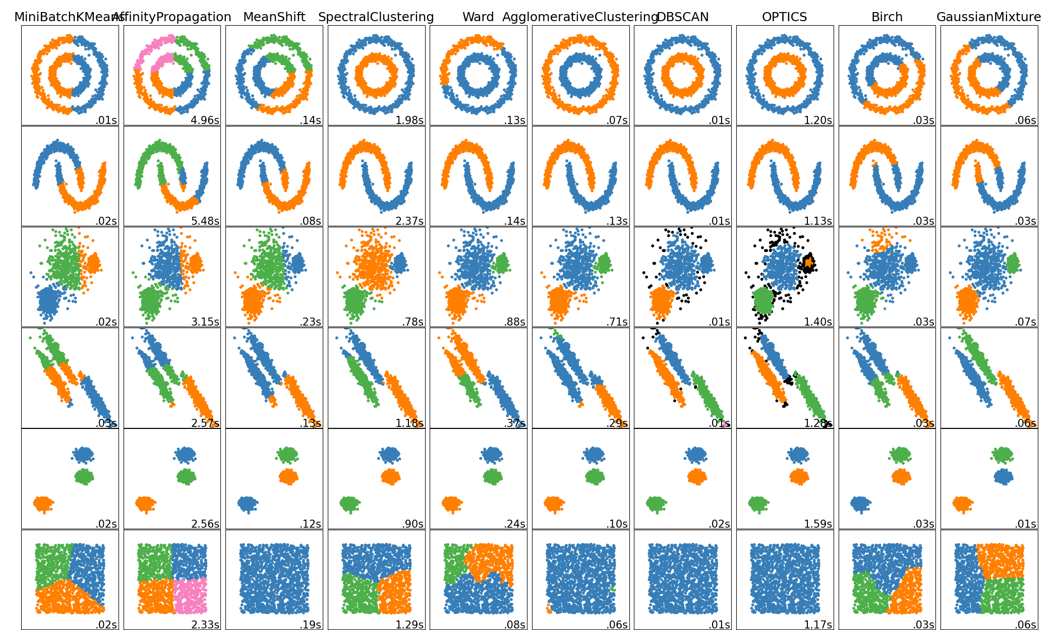
Comparación de diferentes algoritmos de agrupamiento en conjuntos de datos de juguete

Este ejemplo muestra las características de diferentes algoritmos de agrupamiento en conjuntos de datos «interesantes» pero todavía en 2D. Con la excepción del último conjunto de datos, los parámetros de cada uno de estos pares conjunto de datos-algoritmo se han ajustado para producir buenos resultados de agrupamiento. Algunos algoritmos son más sensibles a los valores de los parámetros que otros.

El último conjunto de datos es un ejemplo de una situación “nula” para el agrupamiento: los datos son homogéneos y no hay un buen conglomeradi. Para este ejemplo, el conjunto de datos nulo utiliza los mismos parámetros que el conjunto de datos de la fila anterior, lo que representa un desajuste en los valores de los parámetros y la estructura de los datos.

Si bien estos ejemplos permiten intuir los algoritmos, esta intuición podría no aplicarse a datos de dimensiones muy altas.

Out:

/home/mapologo/miniconda3/envs/sklearn/lib/python3.9/site-packages/scikit_learn-0.24.1-py3.9-linux-x86_64.egg/sklearn/cluster/_affinity_propagation.py:148: FutureWarning: 'random_state' has been introduced in 0.23. It will be set to None starting from 1.0 (renaming of 0.25) which means that results will differ at every function call. Set 'random_state' to None to silence this warning, or to 0 to keep the behavior of versions <0.23.
  warnings.warn(
/home/mapologo/miniconda3/envs/sklearn/lib/python3.9/site-packages/scikit_learn-0.24.1-py3.9-linux-x86_64.egg/sklearn/cluster/_affinity_propagation.py:148: FutureWarning: 'random_state' has been introduced in 0.23. It will be set to None starting from 1.0 (renaming of 0.25) which means that results will differ at every function call. Set 'random_state' to None to silence this warning, or to 0 to keep the behavior of versions <0.23.
  warnings.warn(
/home/mapologo/miniconda3/envs/sklearn/lib/python3.9/site-packages/scikit_learn-0.24.1-py3.9-linux-x86_64.egg/sklearn/cluster/_affinity_propagation.py:148: FutureWarning: 'random_state' has been introduced in 0.23. It will be set to None starting from 1.0 (renaming of 0.25) which means that results will differ at every function call. Set 'random_state' to None to silence this warning, or to 0 to keep the behavior of versions <0.23.
  warnings.warn(
/home/mapologo/miniconda3/envs/sklearn/lib/python3.9/site-packages/scikit_learn-0.24.1-py3.9-linux-x86_64.egg/sklearn/cluster/_affinity_propagation.py:148: FutureWarning: 'random_state' has been introduced in 0.23. It will be set to None starting from 1.0 (renaming of 0.25) which means that results will differ at every function call. Set 'random_state' to None to silence this warning, or to 0 to keep the behavior of versions <0.23.
  warnings.warn(
/home/mapologo/miniconda3/envs/sklearn/lib/python3.9/site-packages/scikit_learn-0.24.1-py3.9-linux-x86_64.egg/sklearn/cluster/_affinity_propagation.py:148: FutureWarning: 'random_state' has been introduced in 0.23. It will be set to None starting from 1.0 (renaming of 0.25) which means that results will differ at every function call. Set 'random_state' to None to silence this warning, or to 0 to keep the behavior of versions <0.23.
  warnings.warn(
/home/mapologo/miniconda3/envs/sklearn/lib/python3.9/site-packages/scikit_learn-0.24.1-py3.9-linux-x86_64.egg/sklearn/cluster/_affinity_propagation.py:148: FutureWarning: 'random_state' has been introduced in 0.23. It will be set to None starting from 1.0 (renaming of 0.25) which means that results will differ at every function call. Set 'random_state' to None to silence this warning, or to 0 to keep the behavior of versions <0.23.
  warnings.warn(

print(__doc__)

import time
import warnings

import numpy as np
import matplotlib.pyplot as plt

from sklearn import cluster, datasets, mixture
from sklearn.neighbors import kneighbors_graph
from sklearn.preprocessing import StandardScaler
from itertools import cycle, islice

np.random.seed(0)

# ============
# Generate datasets. We choose the size big enough to see the scalability
# of the algorithms, but not too big to avoid too long running times
# ============
n_samples = 1500
noisy_circles = datasets.make_circles(n_samples=n_samples, factor=.5,
                                      noise=.05)
noisy_moons = datasets.make_moons(n_samples=n_samples, noise=.05)
blobs = datasets.make_blobs(n_samples=n_samples, random_state=8)
no_structure = np.random.rand(n_samples, 2), None

# Anisotropicly distributed data
random_state = 170
X, y = datasets.make_blobs(n_samples=n_samples, random_state=random_state)
transformation = [[0.6, -0.6], [-0.4, 0.8]]
X_aniso = np.dot(X, transformation)
aniso = (X_aniso, y)

# blobs with varied variances
varied = datasets.make_blobs(n_samples=n_samples,
                             cluster_std=[1.0, 2.5, 0.5],
                             random_state=random_state)

# ============
# Set up cluster parameters
# ============
plt.figure(figsize=(9 * 2 + 3, 12.5))
plt.subplots_adjust(left=.02, right=.98, bottom=.001, top=.96, wspace=.05,
                    hspace=.01)

plot_num = 1

default_base = {'quantile': .3,
                'eps': .3,
                'damping': .9,
                'preference': -200,
                'n_neighbors': 10,
                'n_clusters': 3,
                'min_samples': 20,
                'xi': 0.05,
                'min_cluster_size': 0.1}

datasets = [
    (noisy_circles, {'damping': .77, 'preference': -240,
                     'quantile': .2, 'n_clusters': 2,
                     'min_samples': 20, 'xi': 0.25}),
    (noisy_moons, {'damping': .75, 'preference': -220, 'n_clusters': 2}),
    (varied, {'eps': .18, 'n_neighbors': 2,
              'min_samples': 5, 'xi': 0.035, 'min_cluster_size': .2}),
    (aniso, {'eps': .15, 'n_neighbors': 2,
             'min_samples': 20, 'xi': 0.1, 'min_cluster_size': .2}),
    (blobs, {}),
    (no_structure, {})]

for i_dataset, (dataset, algo_params) in enumerate(datasets):
    # update parameters with dataset-specific values
    params = default_base.copy()
    params.update(algo_params)

    X, y = dataset

    # normalize dataset for easier parameter selection
    X = StandardScaler().fit_transform(X)

    # estimate bandwidth for mean shift
    bandwidth = cluster.estimate_bandwidth(X, quantile=params['quantile'])

    # connectivity matrix for structured Ward
    connectivity = kneighbors_graph(
        X, n_neighbors=params['n_neighbors'], include_self=False)
    # make connectivity symmetric
    connectivity = 0.5 * (connectivity + connectivity.T)

    # ============
    # Create cluster objects
    # ============
    ms = cluster.MeanShift(bandwidth=bandwidth, bin_seeding=True)
    two_means = cluster.MiniBatchKMeans(n_clusters=params['n_clusters'])
    ward = cluster.AgglomerativeClustering(
        n_clusters=params['n_clusters'], linkage='ward',
        connectivity=connectivity)
    spectral = cluster.SpectralClustering(
        n_clusters=params['n_clusters'], eigen_solver='arpack',
        affinity="nearest_neighbors")
    dbscan = cluster.DBSCAN(eps=params['eps'])
    optics = cluster.OPTICS(min_samples=params['min_samples'],
                            xi=params['xi'],
                            min_cluster_size=params['min_cluster_size'])
    affinity_propagation = cluster.AffinityPropagation(
        damping=params['damping'], preference=params['preference'])
    average_linkage = cluster.AgglomerativeClustering(
        linkage="average", affinity="cityblock",
        n_clusters=params['n_clusters'], connectivity=connectivity)
    birch = cluster.Birch(n_clusters=params['n_clusters'])
    gmm = mixture.GaussianMixture(
        n_components=params['n_clusters'], covariance_type='full')

    clustering_algorithms = (
        ('MiniBatchKMeans', two_means),
        ('AffinityPropagation', affinity_propagation),
        ('MeanShift', ms),
        ('SpectralClustering', spectral),
        ('Ward', ward),
        ('AgglomerativeClustering', average_linkage),
        ('DBSCAN', dbscan),
        ('OPTICS', optics),
        ('Birch', birch),
        ('GaussianMixture', gmm)
    )

    for name, algorithm in clustering_algorithms:
        t0 = time.time()

        # catch warnings related to kneighbors_graph
        with warnings.catch_warnings():
            warnings.filterwarnings(
                "ignore",
                message="the number of connected components of the " +
                "connectivity matrix is [0-9]{1,2}" +
                " > 1. Completing it to avoid stopping the tree early.",
                category=UserWarning)
            warnings.filterwarnings(
                "ignore",
                message="Graph is not fully connected, spectral embedding" +
                " may not work as expected.",
                category=UserWarning)
            algorithm.fit(X)

        t1 = time.time()
        if hasattr(algorithm, 'labels_'):
            y_pred = algorithm.labels_.astype(int)
        else:
            y_pred = algorithm.predict(X)

        plt.subplot(len(datasets), len(clustering_algorithms), plot_num)
        if i_dataset == 0:
            plt.title(name, size=18)

        colors = np.array(list(islice(cycle(['#377eb8', '#ff7f00', '#4daf4a',
                                             '#f781bf', '#a65628', '#984ea3',
                                             '#999999', '#e41a1c', '#dede00']),
                                      int(max(y_pred) + 1))))
        # add black color for outliers (if any)
        colors = np.append(colors, ["#000000"])
        plt.scatter(X[:, 0], X[:, 1], s=10, color=colors[y_pred])

        plt.xlim(-2.5, 2.5)
        plt.ylim(-2.5, 2.5)
        plt.xticks(())
        plt.yticks(())
        plt.text(.99, .01, ('%.2fs' % (t1 - t0)).lstrip('0'),
                 transform=plt.gca().transAxes, size=15,
                 horizontalalignment='right')
        plot_num += 1

plt.show()