Visualización de la estructura bursátil

Este ejemplo emplea varias técnicas de aprendizaje no supervisado para extraer la estructura del mercado de valores a partir de las variaciones en las cotizaciones históricas.

La cantidad que utilizamos es la variación diaria del precio de las cotizaciones: las cotizaciones que están vinculadas tienden a cofluir durante un día.

Aprendizaje de la estructura del grafo

Utilizamos la estimación de la covarianza inversa dispersa para encontrar qué cotizaciones están correlacionadas condicionalmente con las demás. En concreto, la covarianza inversa dispersa nos da un gráfico, que es una lista de conexión. Para cada símbolo, los símbolos con los que está conectado son los que sirven para explicar sus fluctuaciones.

Análisis de conglomerados

Utilizamos el clustering para agrupar las cotizaciones que se comportan de forma similar. Aquí, entre las varias técnicas de clustering disponibles en scikit-learn, utilizamos Propagación de la afinidad ya que no impone clusters de igual tamaño, y puede elegir automáticamente el número de clusters a partir de los datos.

Observa que esto nos da una indicación diferente a la del gráfico, ya que el gráfico refleja las relaciones condicionales entre las variables, mientras que la agrupación refleja las propiedades marginales: se puede considerar que las variables agrupadas tienen un impacto similar a nivel de toda la bolsa.

Incrustación en el espacio 2D

Para la visualización, necesitamos disponer los diferentes símbolos en un lienzo 2D. Para ello, utilizamos técnicas de Aprendizaje múltiple para recuperar la incrustación en 2D.

Visualización

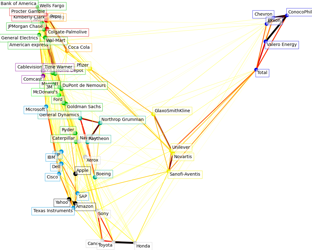
Los resultados de los 3 modelos se combinan en un gráfico 2D en el que los nodos representan las poblaciones y las aristas las:

• las etiquetas de los clusters se utilizan para definir el color de los nodos

• el modelo de covarianza dispersa se utiliza para mostrar la fuerza de los bordes

• la incrustación 2D se utiliza para posicionar los nodos en el plano

Este ejemplo tiene una buena cantidad de código relacionado con la visualización, ya que la visualización es crucial aquí para mostrar el gráfico. Uno de los retos es posicionar las etiquetas minimizando el solapamiento. Para ello utilizamos una heurística basada en la dirección del vecino más cercano a lo largo de cada eje.

Out:

Fetching quote history for 'AAPL'
Fetching quote history for 'AIG'
Fetching quote history for 'AMZN'
Fetching quote history for 'AXP'
Fetching quote history for 'BA'
Fetching quote history for 'BAC'
Fetching quote history for 'CAJ'
Fetching quote history for 'CAT'
Fetching quote history for 'CL'
Fetching quote history for 'CMCSA'
Fetching quote history for 'COP'
Fetching quote history for 'CSCO'
Fetching quote history for 'CVC'
Fetching quote history for 'CVS'
Fetching quote history for 'CVX'
Fetching quote history for 'DD'
Fetching quote history for 'DELL'
Fetching quote history for 'F'
Fetching quote history for 'GD'
Fetching quote history for 'GE'
Fetching quote history for 'GS'
Fetching quote history for 'GSK'
Fetching quote history for 'HD'
Fetching quote history for 'HMC'
Fetching quote history for 'HPQ'
Fetching quote history for 'IBM'
Fetching quote history for 'JPM'
Fetching quote history for 'K'
Fetching quote history for 'KMB'
Fetching quote history for 'KO'
Fetching quote history for 'MAR'
Fetching quote history for 'MCD'
Fetching quote history for 'MMM'
Fetching quote history for 'MSFT'
Fetching quote history for 'NAV'
Fetching quote history for 'NOC'
Fetching quote history for 'NVS'
Fetching quote history for 'PEP'
Fetching quote history for 'PFE'
Fetching quote history for 'PG'
Fetching quote history for 'R'
Fetching quote history for 'RTN'
Fetching quote history for 'SAP'
Fetching quote history for 'SNE'
Fetching quote history for 'SNY'
Fetching quote history for 'TM'
Fetching quote history for 'TOT'
Fetching quote history for 'TWX'
Fetching quote history for 'TXN'
Fetching quote history for 'UN'
Fetching quote history for 'VLO'
Fetching quote history for 'WFC'
Fetching quote history for 'WMT'
Fetching quote history for 'XOM'
Fetching quote history for 'XRX'
Fetching quote history for 'YHOO'
/home/mapologo/miniconda3/envs/sklearn/lib/python3.9/site-packages/numpy/core/_methods.py:229: RuntimeWarning: invalid value encountered in subtract
  x = asanyarray(arr - arrmean)
Cluster 1: Apple, Amazon, Yahoo
Cluster 2: Comcast, Cablevision, Time Warner
Cluster 3: ConocoPhillips, Chevron, Total, Valero Energy, Exxon
Cluster 4: Cisco, Dell, HP, IBM, Microsoft, SAP, Texas Instruments
Cluster 5: Boeing, General Dynamics, Northrop Grumman, Raytheon
Cluster 6: AIG, American express, Bank of America, Caterpillar, CVS, DuPont de Nemours, Ford, General Electrics, Goldman Sachs, Home Depot, JPMorgan Chase, Marriott, 3M, Ryder, Wells Fargo, Wal-Mart
Cluster 7: McDonald's
Cluster 8: GlaxoSmithKline, Novartis, Pfizer, Sanofi-Aventis, Unilever
Cluster 9: Kellogg, Coca Cola, Pepsi
Cluster 10: Colgate-Palmolive, Kimberly-Clark, Procter Gamble
Cluster 11: Canon, Honda, Navistar, Sony, Toyota, Xerox

# Author: Gael Varoquaux gael.varoquaux@normalesup.org
# License: BSD 3 clause

import sys

import numpy as np
import matplotlib.pyplot as plt
from matplotlib.collections import LineCollection

import pandas as pd

from sklearn import cluster, covariance, manifold

print(__doc__)


# #############################################################################
# Retrieve the data from Internet

# The data is from 2003 - 2008. This is reasonably calm: (not too long ago so
# that we get high-tech firms, and before the 2008 crash). This kind of
# historical data can be obtained for from APIs like the quandl.com and
# alphavantage.co ones.

symbol_dict = {
    'TOT': 'Total',
    'XOM': 'Exxon',
    'CVX': 'Chevron',
    'COP': 'ConocoPhillips',
    'VLO': 'Valero Energy',
    'MSFT': 'Microsoft',
    'IBM': 'IBM',
    'TWX': 'Time Warner',
    'CMCSA': 'Comcast',
    'CVC': 'Cablevision',
    'YHOO': 'Yahoo',
    'DELL': 'Dell',
    'HPQ': 'HP',
    'AMZN': 'Amazon',
    'TM': 'Toyota',
    'CAJ': 'Canon',
    'SNE': 'Sony',
    'F': 'Ford',
    'HMC': 'Honda',
    'NAV': 'Navistar',
    'NOC': 'Northrop Grumman',
    'BA': 'Boeing',
    'KO': 'Coca Cola',
    'MMM': '3M',
    'MCD': 'McDonald\'s',
    'PEP': 'Pepsi',
    'K': 'Kellogg',
    'UN': 'Unilever',
    'MAR': 'Marriott',
    'PG': 'Procter Gamble',
    'CL': 'Colgate-Palmolive',
    'GE': 'General Electrics',
    'WFC': 'Wells Fargo',
    'JPM': 'JPMorgan Chase',
    'AIG': 'AIG',
    'AXP': 'American express',
    'BAC': 'Bank of America',
    'GS': 'Goldman Sachs',
    'AAPL': 'Apple',
    'SAP': 'SAP',
    'CSCO': 'Cisco',
    'TXN': 'Texas Instruments',
    'XRX': 'Xerox',
    'WMT': 'Wal-Mart',
    'HD': 'Home Depot',
    'GSK': 'GlaxoSmithKline',
    'PFE': 'Pfizer',
    'SNY': 'Sanofi-Aventis',
    'NVS': 'Novartis',
    'KMB': 'Kimberly-Clark',
    'R': 'Ryder',
    'GD': 'General Dynamics',
    'RTN': 'Raytheon',
    'CVS': 'CVS',
    'CAT': 'Caterpillar',
    'DD': 'DuPont de Nemours'}


symbols, names = np.array(sorted(symbol_dict.items())).T

quotes = []

for symbol in symbols:
    print('Fetching quote history for %r' % symbol, file=sys.stderr)
    url = ('https://raw.githubusercontent.com/scikit-learn/examples-data/'
           'master/financial-data/{}.csv')
    quotes.append(pd.read_csv(url.format(symbol)))

close_prices = np.vstack([q['close'] for q in quotes])
open_prices = np.vstack([q['open'] for q in quotes])

# The daily variations of the quotes are what carry most information
variation = close_prices - open_prices


# #############################################################################
# Learn a graphical structure from the correlations
edge_model = covariance.GraphicalLassoCV()

# standardize the time series: using correlations rather than covariance
# is more efficient for structure recovery
X = variation.copy().T
X /= X.std(axis=0)
edge_model.fit(X)

# #############################################################################
# Cluster using affinity propagation

_, labels = cluster.affinity_propagation(edge_model.covariance_,
                                         random_state=0)
n_labels = labels.max()

for i in range(n_labels + 1):
    print('Cluster %i: %s' % ((i + 1), ', '.join(names[labels == i])))

# #############################################################################
# Find a low-dimension embedding for visualization: find the best position of
# the nodes (the stocks) on a 2D plane

# We use a dense eigen_solver to achieve reproducibility (arpack is
# initiated with random vectors that we don't control). In addition, we
# use a large number of neighbors to capture the large-scale structure.
node_position_model = manifold.LocallyLinearEmbedding(
    n_components=2, eigen_solver='dense', n_neighbors=6)

embedding = node_position_model.fit_transform(X.T).T

# #############################################################################
# Visualization
plt.figure(1, facecolor='w', figsize=(10, 8))
plt.clf()
ax = plt.axes([0., 0., 1., 1.])
plt.axis('off')

# Display a graph of the partial correlations
partial_correlations = edge_model.precision_.copy()
d = 1 / np.sqrt(np.diag(partial_correlations))
partial_correlations *= d
partial_correlations *= d[:, np.newaxis]
non_zero = (np.abs(np.triu(partial_correlations, k=1)) > 0.02)

# Plot the nodes using the coordinates of our embedding
plt.scatter(embedding[0], embedding[1], s=100 * d ** 2, c=labels,
            cmap=plt.cm.nipy_spectral)

# Plot the edges
start_idx, end_idx = np.where(non_zero)
# a sequence of (*line0*, *line1*, *line2*), where::
#            linen = (x0, y0), (x1, y1), ... (xm, ym)
segments = [[embedding[:, start], embedding[:, stop]]
            for start, stop in zip(start_idx, end_idx)]
values = np.abs(partial_correlations[non_zero])
lc = LineCollection(segments,
                    zorder=0, cmap=plt.cm.hot_r,
                    norm=plt.Normalize(0, .7 * values.max()))
lc.set_array(values)
lc.set_linewidths(15 * values)
ax.add_collection(lc)

# Add a label to each node. The challenge here is that we want to
# position the labels to avoid overlap with other labels
for index, (name, label, (x, y)) in enumerate(
        zip(names, labels, embedding.T)):

    dx = x - embedding[0]
    dx[index] = 1
    dy = y - embedding[1]
    dy[index] = 1
    this_dx = dx[np.argmin(np.abs(dy))]
    this_dy = dy[np.argmin(np.abs(dx))]
    if this_dx > 0:
        horizontalalignment = 'left'
        x = x + .002
    else:
        horizontalalignment = 'right'
        x = x - .002
    if this_dy > 0:
        verticalalignment = 'bottom'
        y = y + .002
    else:
        verticalalignment = 'top'
        y = y - .002
    plt.text(x, y, name, size=10,
             horizontalalignment=horizontalalignment,
             verticalalignment=verticalalignment,
             bbox=dict(facecolor='w',
                       edgecolor=plt.cm.nipy_spectral(label / float(n_labels)),
                       alpha=.6))

plt.xlim(embedding[0].min() - .15 * embedding[0].ptp(),
         embedding[0].max() + .10 * embedding[0].ptp(),)
plt.ylim(embedding[1].min() - .03 * embedding[1].ptp(),
         embedding[1].max() + .03 * embedding[1].ptp())

plt.show()