Clasificación de documentos de texto fuera del núcleo

Este es un ejemplo que muestra cómo scikit-learn puede ser utilizado para la clasificación utilizando un enfoque fuera del núcleo: el aprendizaje de los datos que no caben en la memoria principal. Hacemos uso de un clasificador en línea, es decir, uno que soporta el método partial_fit, que será alimentado con lotes de ejemplos. Para garantizar que el espacio de características siga siendo el mismo a lo largo del tiempo, aprovechamos un HashingVectorizer que proyectará cada ejemplo en el mismo espacio de características. Esto es especialmente útil en el caso de la clasificación de textos, donde pueden aparecer nuevas características (palabras) en cada lote.

# Authors: Eustache Diemert <eustache@diemert.fr>
#          @FedericoV <https://github.com/FedericoV/>
# License: BSD 3 clause

from glob import glob
import itertools
import os.path
import re
import tarfile
import time
import sys

import numpy as np
import matplotlib.pyplot as plt
from matplotlib import rcParams

from html.parser import HTMLParser
from urllib.request import urlretrieve
from sklearn.datasets import get_data_home
from sklearn.feature_extraction.text import HashingVectorizer
from sklearn.linear_model import SGDClassifier
from sklearn.linear_model import PassiveAggressiveClassifier
from sklearn.linear_model import Perceptron
from sklearn.naive_bayes import MultinomialNB


def _not_in_sphinx():
    # Hack to detect whether we are running by the sphinx builder
    return '__file__' in globals()

Rutinas relacionadas con los datos de Reuters

El conjunto de datos utilizado en este ejemplo es Reuters-21578 proporcionado por el repositorio UCI ML. Se descargará automáticamente y se descomprimirá en la primera ejecución.

class ReutersParser(HTMLParser):
    """Utility class to parse a SGML file and yield documents one at a time."""

    def __init__(self, encoding='latin-1'):
        HTMLParser.__init__(self)
        self._reset()
        self.encoding = encoding

    def handle_starttag(self, tag, attrs):
        method = 'start_' + tag
        getattr(self, method, lambda x: None)(attrs)

    def handle_endtag(self, tag):
        method = 'end_' + tag
        getattr(self, method, lambda: None)()

    def _reset(self):
        self.in_title = 0
        self.in_body = 0
        self.in_topics = 0
        self.in_topic_d = 0
        self.title = ""
        self.body = ""
        self.topics = []
        self.topic_d = ""

    def parse(self, fd):
        self.docs = []
        for chunk in fd:
            self.feed(chunk.decode(self.encoding))
            for doc in self.docs:
                yield doc
            self.docs = []
        self.close()

    def handle_data(self, data):
        if self.in_body:
            self.body += data
        elif self.in_title:
            self.title += data
        elif self.in_topic_d:
            self.topic_d += data

    def start_reuters(self, attributes):
        pass

    def end_reuters(self):
        self.body = re.sub(r'\s+', r' ', self.body)
        self.docs.append({'title': self.title,
                          'body': self.body,
                          'topics': self.topics})
        self._reset()

    def start_title(self, attributes):
        self.in_title = 1

    def end_title(self):
        self.in_title = 0

    def start_body(self, attributes):
        self.in_body = 1

    def end_body(self):
        self.in_body = 0

    def start_topics(self, attributes):
        self.in_topics = 1

    def end_topics(self):
        self.in_topics = 0

    def start_d(self, attributes):
        self.in_topic_d = 1

    def end_d(self):
        self.in_topic_d = 0
        self.topics.append(self.topic_d)
        self.topic_d = ""


def stream_reuters_documents(data_path=None):
    """Iterate over documents of the Reuters dataset.

    The Reuters archive will automatically be downloaded and uncompressed if
    the `data_path` directory does not exist.

    Documents are represented as dictionaries with 'body' (str),
    'title' (str), 'topics' (list(str)) keys.

    """

    DOWNLOAD_URL = ('http://archive.ics.uci.edu/ml/machine-learning-databases/'
                    'reuters21578-mld/reuters21578.tar.gz')
    ARCHIVE_FILENAME = 'reuters21578.tar.gz'

    if data_path is None:
        data_path = os.path.join(get_data_home(), "reuters")
    if not os.path.exists(data_path):
        """Download the dataset."""
        print("downloading dataset (once and for all) into %s" %
              data_path)
        os.mkdir(data_path)

        def progress(blocknum, bs, size):
            total_sz_mb = '%.2f MB' % (size / 1e6)
            current_sz_mb = '%.2f MB' % ((blocknum * bs) / 1e6)
            if _not_in_sphinx():
                sys.stdout.write(
                    '\rdownloaded %s / %s' % (current_sz_mb, total_sz_mb))

        archive_path = os.path.join(data_path, ARCHIVE_FILENAME)
        urlretrieve(DOWNLOAD_URL, filename=archive_path,
                    reporthook=progress)
        if _not_in_sphinx():
            sys.stdout.write('\r')
        print("untarring Reuters dataset...")
        tarfile.open(archive_path, 'r:gz').extractall(data_path)
        print("done.")

    parser = ReutersParser()
    for filename in glob(os.path.join(data_path, "*.sgm")):
        for doc in parser.parse(open(filename, 'rb')):
            yield doc

Principal

Crear el vectorizador y limitar el número de características a un máximo razonable

vectorizer = HashingVectorizer(decode_error='ignore', n_features=2 ** 18,
                               alternate_sign=False)


# Iterator over parsed Reuters SGML files.
data_stream = stream_reuters_documents()

# We learn a binary classification between the "acq" class and all the others.
# "acq" was chosen as it is more or less evenly distributed in the Reuters
# files. For other datasets, one should take care of creating a test set with
# a realistic portion of positive instances.
all_classes = np.array([0, 1])
positive_class = 'acq'

# Here are some classifiers that support the `partial_fit` method
partial_fit_classifiers = {
    'SGD': SGDClassifier(max_iter=5),
    'Perceptron': Perceptron(),
    'NB Multinomial': MultinomialNB(alpha=0.01),
    'Passive-Aggressive': PassiveAggressiveClassifier(),
}


def get_minibatch(doc_iter, size, pos_class=positive_class):
    """Extract a minibatch of examples, return a tuple X_text, y.

    Note: size is before excluding invalid docs with no topics assigned.

    """
    data = [('{title}\n\n{body}'.format(**doc), pos_class in doc['topics'])
            for doc in itertools.islice(doc_iter, size)
            if doc['topics']]
    if not len(data):
        return np.asarray([], dtype=int), np.asarray([], dtype=int)
    X_text, y = zip(*data)
    return X_text, np.asarray(y, dtype=int)


def iter_minibatches(doc_iter, minibatch_size):
    """Generator of minibatches."""
    X_text, y = get_minibatch(doc_iter, minibatch_size)
    while len(X_text):
        yield X_text, y
        X_text, y = get_minibatch(doc_iter, minibatch_size)


# test data statistics
test_stats = {'n_test': 0, 'n_test_pos': 0}

# First we hold out a number of examples to estimate accuracy
n_test_documents = 1000
tick = time.time()
X_test_text, y_test = get_minibatch(data_stream, 1000)
parsing_time = time.time() - tick
tick = time.time()
X_test = vectorizer.transform(X_test_text)
vectorizing_time = time.time() - tick
test_stats['n_test'] += len(y_test)
test_stats['n_test_pos'] += sum(y_test)
print("Test set is %d documents (%d positive)" % (len(y_test), sum(y_test)))


def progress(cls_name, stats):
    """Report progress information, return a string."""
    duration = time.time() - stats['t0']
    s = "%20s classifier : \t" % cls_name
    s += "%(n_train)6d train docs (%(n_train_pos)6d positive) " % stats
    s += "%(n_test)6d test docs (%(n_test_pos)6d positive) " % test_stats
    s += "accuracy: %(accuracy).3f " % stats
    s += "in %.2fs (%5d docs/s)" % (duration, stats['n_train'] / duration)
    return s


cls_stats = {}

for cls_name in partial_fit_classifiers:
    stats = {'n_train': 0, 'n_train_pos': 0,
             'accuracy': 0.0, 'accuracy_history': [(0, 0)], 't0': time.time(),
             'runtime_history': [(0, 0)], 'total_fit_time': 0.0}
    cls_stats[cls_name] = stats

get_minibatch(data_stream, n_test_documents)
# Discard test set

# We will feed the classifier with mini-batches of 1000 documents; this means
# we have at most 1000 docs in memory at any time.  The smaller the document
# batch, the bigger the relative overhead of the partial fit methods.
minibatch_size = 1000

# Create the data_stream that parses Reuters SGML files and iterates on
# documents as a stream.
minibatch_iterators = iter_minibatches(data_stream, minibatch_size)
total_vect_time = 0.0

# Main loop : iterate on mini-batches of examples
for i, (X_train_text, y_train) in enumerate(minibatch_iterators):

    tick = time.time()
    X_train = vectorizer.transform(X_train_text)
    total_vect_time += time.time() - tick

    for cls_name, cls in partial_fit_classifiers.items():
        tick = time.time()
        # update estimator with examples in the current mini-batch
        cls.partial_fit(X_train, y_train, classes=all_classes)

        # accumulate test accuracy stats
        cls_stats[cls_name]['total_fit_time'] += time.time() - tick
        cls_stats[cls_name]['n_train'] += X_train.shape[0]
        cls_stats[cls_name]['n_train_pos'] += sum(y_train)
        tick = time.time()
        cls_stats[cls_name]['accuracy'] = cls.score(X_test, y_test)
        cls_stats[cls_name]['prediction_time'] = time.time() - tick
        acc_history = (cls_stats[cls_name]['accuracy'],
                       cls_stats[cls_name]['n_train'])
        cls_stats[cls_name]['accuracy_history'].append(acc_history)
        run_history = (cls_stats[cls_name]['accuracy'],
                       total_vect_time + cls_stats[cls_name]['total_fit_time'])
        cls_stats[cls_name]['runtime_history'].append(run_history)

        if i % 3 == 0:
            print(progress(cls_name, cls_stats[cls_name]))
    if i % 3 == 0:
        print('\n')

Out:

downloading dataset (once and for all) into /home/mapologo/scikit_learn_data/reuters
untarring Reuters dataset...
done.
Test set is 986 documents (159 positive)
                 SGD classifier :          955 train docs (    93 positive)    986 test docs (   159 positive) accuracy: 0.896 in 0.75s ( 1269 docs/s)
          Perceptron classifier :          955 train docs (    93 positive)    986 test docs (   159 positive) accuracy: 0.860 in 0.76s ( 1261 docs/s)
      NB Multinomial classifier :          955 train docs (    93 positive)    986 test docs (   159 positive) accuracy: 0.839 in 0.79s ( 1216 docs/s)
  Passive-Aggressive classifier :          955 train docs (    93 positive)    986 test docs (   159 positive) accuracy: 0.914 in 0.79s ( 1209 docs/s)


                 SGD classifier :         3370 train docs (   401 positive)    986 test docs (   159 positive) accuracy: 0.933 in 2.19s ( 1537 docs/s)
          Perceptron classifier :         3370 train docs (   401 positive)    986 test docs (   159 positive) accuracy: 0.919 in 2.20s ( 1534 docs/s)
      NB Multinomial classifier :         3370 train docs (   401 positive)    986 test docs (   159 positive) accuracy: 0.847 in 2.22s ( 1519 docs/s)
  Passive-Aggressive classifier :         3370 train docs (   401 positive)    986 test docs (   159 positive) accuracy: 0.929 in 2.22s ( 1516 docs/s)


                 SGD classifier :         6243 train docs (   840 positive)    986 test docs (   159 positive) accuracy: 0.955 in 3.78s ( 1653 docs/s)
          Perceptron classifier :         6243 train docs (   840 positive)    986 test docs (   159 positive) accuracy: 0.945 in 3.78s ( 1651 docs/s)
      NB Multinomial classifier :         6243 train docs (   840 positive)    986 test docs (   159 positive) accuracy: 0.867 in 3.81s ( 1639 docs/s)
  Passive-Aggressive classifier :         6243 train docs (   840 positive)    986 test docs (   159 positive) accuracy: 0.949 in 3.81s ( 1638 docs/s)


                 SGD classifier :         9060 train docs (  1161 positive)    986 test docs (   159 positive) accuracy: 0.951 in 5.31s ( 1707 docs/s)
          Perceptron classifier :         9060 train docs (  1161 positive)    986 test docs (   159 positive) accuracy: 0.947 in 5.31s ( 1705 docs/s)
      NB Multinomial classifier :         9060 train docs (  1161 positive)    986 test docs (   159 positive) accuracy: 0.896 in 5.33s ( 1698 docs/s)
  Passive-Aggressive classifier :         9060 train docs (  1161 positive)    986 test docs (   159 positive) accuracy: 0.944 in 5.34s ( 1696 docs/s)


                 SGD classifier :        11937 train docs (  1525 positive)    986 test docs (   159 positive) accuracy: 0.928 in 6.80s ( 1756 docs/s)
          Perceptron classifier :        11937 train docs (  1525 positive)    986 test docs (   159 positive) accuracy: 0.946 in 6.80s ( 1754 docs/s)
      NB Multinomial classifier :        11937 train docs (  1525 positive)    986 test docs (   159 positive) accuracy: 0.910 in 6.83s ( 1748 docs/s)
  Passive-Aggressive classifier :        11937 train docs (  1525 positive)    986 test docs (   159 positive) accuracy: 0.960 in 6.83s ( 1747 docs/s)


                 SGD classifier :        14352 train docs (  1822 positive)    986 test docs (   159 positive) accuracy: 0.951 in 8.29s ( 1730 docs/s)
          Perceptron classifier :        14352 train docs (  1822 positive)    986 test docs (   159 positive) accuracy: 0.958 in 8.30s ( 1729 docs/s)
      NB Multinomial classifier :        14352 train docs (  1822 positive)    986 test docs (   159 positive) accuracy: 0.912 in 8.32s ( 1724 docs/s)
  Passive-Aggressive classifier :        14352 train docs (  1822 positive)    986 test docs (   159 positive) accuracy: 0.957 in 8.33s ( 1723 docs/s)


                 SGD classifier :        17184 train docs (  2125 positive)    986 test docs (   159 positive) accuracy: 0.959 in 9.80s ( 1754 docs/s)
          Perceptron classifier :        17184 train docs (  2125 positive)    986 test docs (   159 positive) accuracy: 0.934 in 9.80s ( 1753 docs/s)
      NB Multinomial classifier :        17184 train docs (  2125 positive)    986 test docs (   159 positive) accuracy: 0.912 in 9.82s ( 1749 docs/s)
  Passive-Aggressive classifier :        17184 train docs (  2125 positive)    986 test docs (   159 positive) accuracy: 0.965 in 9.83s ( 1748 docs/s)

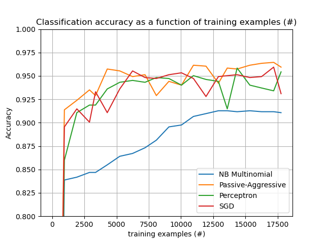
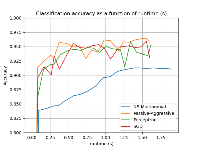
Gráfico de los resultados

El gráfico representa la curva de aprendizaje del clasificador: la evolución de la precisión de la clasificación a lo largo de los minilotes. La precisión se mide en las primeras 1000 muestras, que se mantienen como conjunto de validación.

Para limitar el consumo de memoria, ponemos en cola ejemplos hasta una cantidad fija antes de alimentarlos al aprendiz.

def plot_accuracy(x, y, x_legend):
    """Plot accuracy as a function of x."""
    x = np.array(x)
    y = np.array(y)
    plt.title('Classification accuracy as a function of %s' % x_legend)
    plt.xlabel('%s' % x_legend)
    plt.ylabel('Accuracy')
    plt.grid(True)
    plt.plot(x, y)


rcParams['legend.fontsize'] = 10
cls_names = list(sorted(cls_stats.keys()))

# Plot accuracy evolution
plt.figure()
for _, stats in sorted(cls_stats.items()):
    # Plot accuracy evolution with #examples
    accuracy, n_examples = zip(*stats['accuracy_history'])
    plot_accuracy(n_examples, accuracy, "training examples (#)")
    ax = plt.gca()
    ax.set_ylim((0.8, 1))
plt.legend(cls_names, loc='best')

plt.figure()
for _, stats in sorted(cls_stats.items()):
    # Plot accuracy evolution with runtime
    accuracy, runtime = zip(*stats['runtime_history'])
    plot_accuracy(runtime, accuracy, 'runtime (s)')
    ax = plt.gca()
    ax.set_ylim((0.8, 1))
plt.legend(cls_names, loc='best')

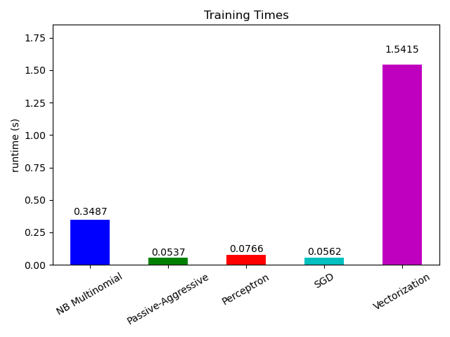
# Plot fitting times
plt.figure()
fig = plt.gcf()
cls_runtime = [stats['total_fit_time']
               for cls_name, stats in sorted(cls_stats.items())]

cls_runtime.append(total_vect_time)
cls_names.append('Vectorization')
bar_colors = ['b', 'g', 'r', 'c', 'm', 'y']

ax = plt.subplot(111)
rectangles = plt.bar(range(len(cls_names)), cls_runtime, width=0.5,
                     color=bar_colors)

ax.set_xticks(np.linspace(0, len(cls_names) - 1, len(cls_names)))
ax.set_xticklabels(cls_names, fontsize=10)
ymax = max(cls_runtime) * 1.2
ax.set_ylim((0, ymax))
ax.set_ylabel('runtime (s)')
ax.set_title('Training Times')


def autolabel(rectangles):
    """attach some text vi autolabel on rectangles."""
    for rect in rectangles:
        height = rect.get_height()
        ax.text(rect.get_x() + rect.get_width() / 2.,
                1.05 * height, '%.4f' % height,
                ha='center', va='bottom')
        plt.setp(plt.xticks()[1], rotation=30)


autolabel(rectangles)
plt.tight_layout()
plt.show()

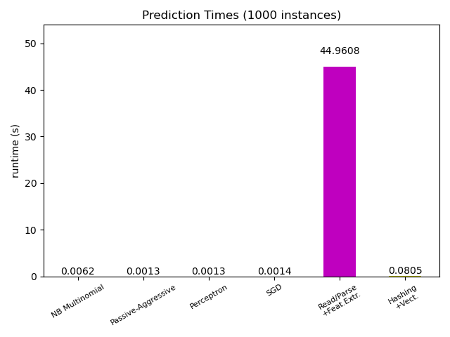
# Plot prediction times
plt.figure()
cls_runtime = []
cls_names = list(sorted(cls_stats.keys()))
for cls_name, stats in sorted(cls_stats.items()):
    cls_runtime.append(stats['prediction_time'])
cls_runtime.append(parsing_time)
cls_names.append('Read/Parse\n+Feat.Extr.')
cls_runtime.append(vectorizing_time)
cls_names.append('Hashing\n+Vect.')

ax = plt.subplot(111)
rectangles = plt.bar(range(len(cls_names)), cls_runtime, width=0.5,
                     color=bar_colors)

ax.set_xticks(np.linspace(0, len(cls_names) - 1, len(cls_names)))
ax.set_xticklabels(cls_names, fontsize=8)
plt.setp(plt.xticks()[1], rotation=30)
ymax = max(cls_runtime) * 1.2
ax.set_ylim((0, ymax))
ax.set_ylabel('runtime (s)')
ax.set_title('Prediction Times (%d instances)' % n_test_documents)
autolabel(rectangles)
plt.tight_layout()
plt.show()

• 
• 
• 
•