Ejemplo de márgenes SVM

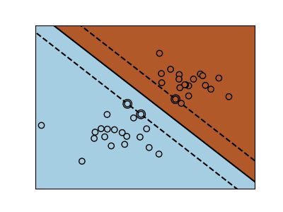
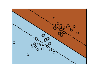
Los gráficos siguientes ilustran el efecto del parámetro C sobre la línea de separación. Un valor grande de C básicamente le dice a nuestro modelo que no tenemos mucha fe en la distribución de nuestros datos, y sólo consideraremos los puntos cercanos a la línea de separación.

Un pequeño valor de C incluye más/todas las observaciones, permitiendo que los márgenes se calculen utilizando todos los datos del área.

• 
• 

Out:

/home/mapologo/Descargas/scikit-learn-0.24.X/examples/svm/plot_svm_margin.py:81: MatplotlibDeprecationWarning: shading='flat' when X and Y have the same dimensions as C is deprecated since 3.3.  Either specify the corners of the quadrilaterals with X and Y, or pass shading='auto', 'nearest' or 'gouraud', or set rcParams['pcolor.shading'].  This will become an error two minor releases later.
  plt.pcolormesh(XX, YY, Z, cmap=plt.cm.Paired)
/home/mapologo/Descargas/scikit-learn-0.24.X/examples/svm/plot_svm_margin.py:81: MatplotlibDeprecationWarning: shading='flat' when X and Y have the same dimensions as C is deprecated since 3.3.  Either specify the corners of the quadrilaterals with X and Y, or pass shading='auto', 'nearest' or 'gouraud', or set rcParams['pcolor.shading'].  This will become an error two minor releases later.
  plt.pcolormesh(XX, YY, Z, cmap=plt.cm.Paired)

print(__doc__)


# Code source: Gaël Varoquaux
# Modified for documentation by Jaques Grobler
# License: BSD 3 clause

import numpy as np
import matplotlib.pyplot as plt
from sklearn import svm

# we create 40 separable points
np.random.seed(0)
X = np.r_[np.random.randn(20, 2) - [2, 2], np.random.randn(20, 2) + [2, 2]]
Y = [0] * 20 + [1] * 20

# figure number
fignum = 1

# fit the model
for name, penalty in (('unreg', 1), ('reg', 0.05)):

    clf = svm.SVC(kernel='linear', C=penalty)
    clf.fit(X, Y)

    # get the separating hyperplane
    w = clf.coef_[0]
    a = -w[0] / w[1]
    xx = np.linspace(-5, 5)
    yy = a * xx - (clf.intercept_[0]) / w[1]

    # plot the parallels to the separating hyperplane that pass through the
    # support vectors (margin away from hyperplane in direction
    # perpendicular to hyperplane). This is sqrt(1+a^2) away vertically in
    # 2-d.
    margin = 1 / np.sqrt(np.sum(clf.coef_ ** 2))
    yy_down = yy - np.sqrt(1 + a ** 2) * margin
    yy_up = yy + np.sqrt(1 + a ** 2) * margin

    # plot the line, the points, and the nearest vectors to the plane
    plt.figure(fignum, figsize=(4, 3))
    plt.clf()
    plt.plot(xx, yy, 'k-')
    plt.plot(xx, yy_down, 'k--')
    plt.plot(xx, yy_up, 'k--')

    plt.scatter(clf.support_vectors_[:, 0], clf.support_vectors_[:, 1], s=80,
                facecolors='none', zorder=10, edgecolors='k')
    plt.scatter(X[:, 0], X[:, 1], c=Y, zorder=10, cmap=plt.cm.Paired,
                edgecolors='k')

    plt.axis('tight')
    x_min = -4.8
    x_max = 4.2
    y_min = -6
    y_max = 6

    XX, YY = np.mgrid[x_min:x_max:200j, y_min:y_max:200j]
    Z = clf.predict(np.c_[XX.ravel(), YY.ravel()])

    # Put the result into a color plot
    Z = Z.reshape(XX.shape)
    plt.figure(fignum, figsize=(4, 3))
    plt.pcolormesh(XX, YY, Z, cmap=plt.cm.Paired)

    plt.xlim(x_min, x_max)
    plt.ylim(y_min, y_max)

    plt.xticks(())
    plt.yticks(())
    fignum = fignum + 1

plt.show()