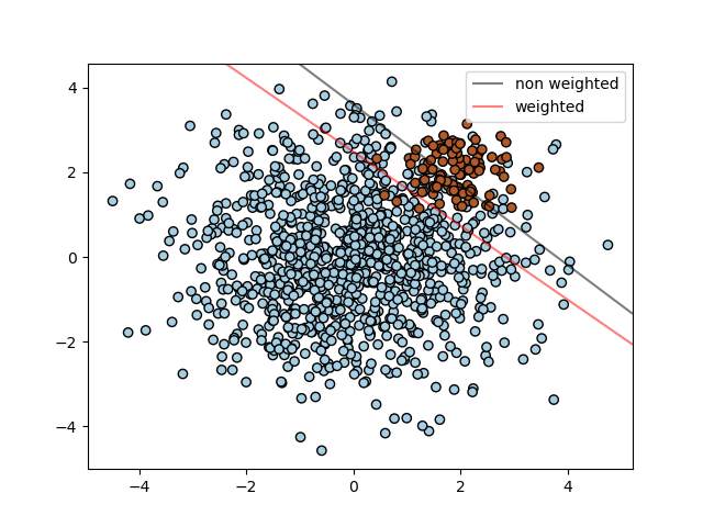
SVM: Hiperplano de separación para clases desequilibradas

Encuentre el hiperplano de separación óptimo utilizando un SVC para las clases que están desequilibradas.

Primero encontramos el plano de separación con un SVC simple y luego trazamos (en guiones) el hiperplano de separación con corrección automática para las clases desequilibradas.

Nota

Este ejemplo también funcionará reemplazando SVC(kernel="linear") con SGDClassifier(loss="hinge"). Establecer el parámetro loss del SGDClassifier igual a hinge producirá un comportamiento como el de un SVC con un núcleo lineal.

Por ejemplo, intenta en lugar del SVC:

clf = SGDClassifier(n_iter=100, alpha=0.01)

print(__doc__)

import numpy as np
import matplotlib.pyplot as plt
from sklearn import svm
from sklearn.datasets import make_blobs

# we create two clusters of random points
n_samples_1 = 1000
n_samples_2 = 100
centers = [[0.0, 0.0], [2.0, 2.0]]
clusters_std = [1.5, 0.5]
X, y = make_blobs(n_samples=[n_samples_1, n_samples_2],
                  centers=centers,
                  cluster_std=clusters_std,
                  random_state=0, shuffle=False)

# fit the model and get the separating hyperplane
clf = svm.SVC(kernel='linear', C=1.0)
clf.fit(X, y)

# fit the model and get the separating hyperplane using weighted classes
wclf = svm.SVC(kernel='linear', class_weight={1: 10})
wclf.fit(X, y)

# plot the samples
plt.scatter(X[:, 0], X[:, 1], c=y, cmap=plt.cm.Paired, edgecolors='k')

# plot the decision functions for both classifiers
ax = plt.gca()
xlim = ax.get_xlim()
ylim = ax.get_ylim()

# create grid to evaluate model
xx = np.linspace(xlim[0], xlim[1], 30)
yy = np.linspace(ylim[0], ylim[1], 30)
YY, XX = np.meshgrid(yy, xx)
xy = np.vstack([XX.ravel(), YY.ravel()]).T

# get the separating hyperplane
Z = clf.decision_function(xy).reshape(XX.shape)

# plot decision boundary and margins
a = ax.contour(XX, YY, Z, colors='k', levels=[0], alpha=0.5, linestyles=['-'])

# get the separating hyperplane for weighted classes
Z = wclf.decision_function(xy).reshape(XX.shape)

# plot decision boundary and margins for weighted classes
b = ax.contour(XX, YY, Z, colors='r', levels=[0], alpha=0.5, linestyles=['-'])

plt.legend([a.collections[0], b.collections[0]], ["non weighted", "weighted"],
           loc="upper right")
plt.show()