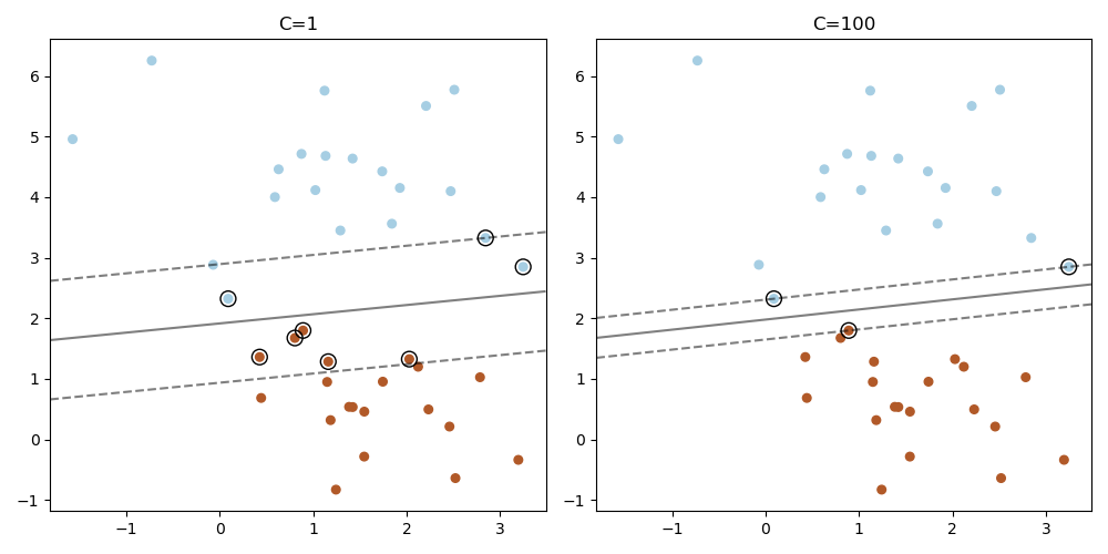
Trazar los vectores de soporte en LinearSVC

A diferencia de SVC (basado en LIBSVM), LinearSVC (basado en LIBLINEAR) no proporciona los vectores soporte. Este ejemplo demuestra cómo obtener los vectores de soporte en LinearSVC.

import numpy as np
import matplotlib.pyplot as plt
from sklearn.datasets import make_blobs
from sklearn.svm import LinearSVC

X, y = make_blobs(n_samples=40, centers=2, random_state=0)

plt.figure(figsize=(10, 5))
for i, C in enumerate([1, 100]):
    # "hinge" is the standard SVM loss
    clf = LinearSVC(C=C, loss="hinge", random_state=42).fit(X, y)
    # obtain the support vectors through the decision function
    decision_function = clf.decision_function(X)
    # we can also calculate the decision function manually
    # decision_function = np.dot(X, clf.coef_[0]) + clf.intercept_[0]
    # The support vectors are the samples that lie within the margin
    # boundaries, whose size is conventionally constrained to 1
    support_vector_indices = np.where(
        np.abs(decision_function) <= 1 + 1e-15)[0]
    support_vectors = X[support_vector_indices]

    plt.subplot(1, 2, i + 1)
    plt.scatter(X[:, 0], X[:, 1], c=y, s=30, cmap=plt.cm.Paired)
    ax = plt.gca()
    xlim = ax.get_xlim()
    ylim = ax.get_ylim()
    xx, yy = np.meshgrid(np.linspace(xlim[0], xlim[1], 50),
                         np.linspace(ylim[0], ylim[1], 50))
    Z = clf.decision_function(np.c_[xx.ravel(), yy.ravel()])
    Z = Z.reshape(xx.shape)
    plt.contour(xx, yy, Z, colors='k', levels=[-1, 0, 1], alpha=0.5,
                linestyles=['--', '-', '--'])
    plt.scatter(support_vectors[:, 0], support_vectors[:, 1], s=100,
                linewidth=1, facecolors='none', edgecolors='k')
    plt.title("C=" + str(C))
plt.tight_layout()
plt.show()