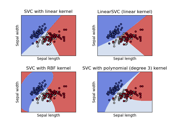
Traza diferentes clasificadores SVM en el conjunto de datos iris

Comparación de diferentes clasificadores SVM lineales en una proyección 2D del conjunto de datos iris. Sólo tenemos en cuenta las dos primeras características de este conjunto de datos:

• Longitud del sepal

• Ancho del sepal

Este ejemplo muestra cómo trazar la superficie de decisión para cuatro clasificadores SVM con diferentes núcleos.

Los modelos lineales LinearSVC() y SVC(kernel='linear') producen límites de decisión ligeramente diferentes. Esto puede ser una consecuencia de las siguientes diferencias:

• LinearSVC minimiza la pérdida de bisagra al cuadrado mientras que SVC minimiza la pérdida de bisagra regular.

• LinearSVC utiliza la reducción multiclase Uno-vs-Todos (también conocida como Uno-vs-Resto) mientras que SVC utiliza la reducción multiclase Uno-vs-Uno.

Ambos modelos lineales tienen límites de decisión lineales (hiperplano intersectorial) mientras que los modelos no lineales del núcleo (polinomio o Gaussian RBF) tienen límites de decisión no lineales más flexibles con formas que dependen del tipo de núcleo y sus parámetros.

Nota

si bien el trazado de la función de decisión de los clasificadores para conjuntos de datos 2D de juguete puede ayudar a obtener una comprensión intuitiva de su respectivo poder expresivo, ten en cuenta que esas intuiciones no siempre se generalizan a problemas más realistas de alta dimensión.

print(__doc__)

import numpy as np
import matplotlib.pyplot as plt
from sklearn import svm, datasets


def make_meshgrid(x, y, h=.02):
    """Create a mesh of points to plot in

    Parameters
    ----------
    x: data to base x-axis meshgrid on
    y: data to base y-axis meshgrid on
    h: stepsize for meshgrid, optional

    Returns
    -------
    xx, yy : ndarray
    """
    x_min, x_max = x.min() - 1, x.max() + 1
    y_min, y_max = y.min() - 1, y.max() + 1
    xx, yy = np.meshgrid(np.arange(x_min, x_max, h),
                         np.arange(y_min, y_max, h))
    return xx, yy


def plot_contours(ax, clf, xx, yy, **params):
    """Plot the decision boundaries for a classifier.

    Parameters
    ----------
    ax: matplotlib axes object
    clf: a classifier
    xx: meshgrid ndarray
    yy: meshgrid ndarray
    params: dictionary of params to pass to contourf, optional
    """
    Z = clf.predict(np.c_[xx.ravel(), yy.ravel()])
    Z = Z.reshape(xx.shape)
    out = ax.contourf(xx, yy, Z, **params)
    return out


# import some data to play with
iris = datasets.load_iris()
# Take the first two features. We could avoid this by using a two-dim dataset
X = iris.data[:, :2]
y = iris.target

# we create an instance of SVM and fit out data. We do not scale our
# data since we want to plot the support vectors
C = 1.0  # SVM regularization parameter
models = (svm.SVC(kernel='linear', C=C),
          svm.LinearSVC(C=C, max_iter=10000),
          svm.SVC(kernel='rbf', gamma=0.7, C=C),
          svm.SVC(kernel='poly', degree=3, gamma='auto', C=C))
models = (clf.fit(X, y) for clf in models)

# title for the plots
titles = ('SVC with linear kernel',
          'LinearSVC (linear kernel)',
          'SVC with RBF kernel',
          'SVC with polynomial (degree 3) kernel')

# Set-up 2x2 grid for plotting.
fig, sub = plt.subplots(2, 2)
plt.subplots_adjust(wspace=0.4, hspace=0.4)

X0, X1 = X[:, 0], X[:, 1]
xx, yy = make_meshgrid(X0, X1)

for clf, title, ax in zip(models, titles, sub.flatten()):
    plot_contours(ax, clf, xx, yy,
                  cmap=plt.cm.coolwarm, alpha=0.8)
    ax.scatter(X0, X1, c=y, cmap=plt.cm.coolwarm, s=20, edgecolors='k')
    ax.set_xlim(xx.min(), xx.max())
    ax.set_ylim(yy.min(), yy.max())
    ax.set_xlabel('Sepal length')
    ax.set_ylabel('Sepal width')
    ax.set_xticks(())
    ax.set_yticks(())
    ax.set_title(title)

plt.show()