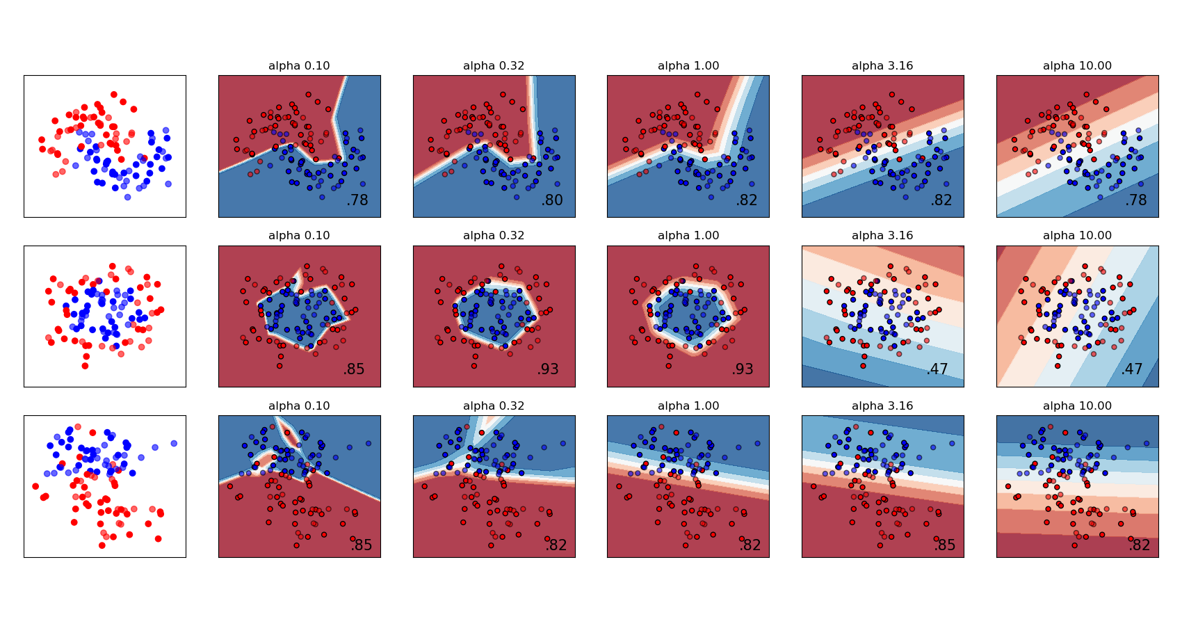
Regularización Variable en el Perceptrón Multicapa

Comparación de diferentes valores del parámetro de regularización “alpha” en conjuntos de datos sintéticos. El gráfico muestra que diferentes alfas dan lugar a diferentes funciones de decisión.

Alpha es un parámetro para el término de regularización, también conocido como término de penalización, que combate el sobreajuste restringiendo el tamaño de los pesos. Aumentar alpha puede corregir una alta varianza (un signo de sobreajuste) fomentando ponderaciones más pequeñas, lo que resulta en un gráfico de frontera de decisión que aparece con menores curvaturas. Del mismo modo, la disminución de alpha puede corregir un sesgo elevado (un signo de subajuste) fomentando ponderaciones más grandes, lo que puede dar lugar a una frontera de decisión más complicada.

print(__doc__)


# Author: Issam H. Laradji
# License: BSD 3 clause

import numpy as np
from matplotlib import pyplot as plt
from matplotlib.colors import ListedColormap
from sklearn.model_selection import train_test_split
from sklearn.preprocessing import StandardScaler
from sklearn.datasets import make_moons, make_circles, make_classification
from sklearn.neural_network import MLPClassifier
from sklearn.pipeline import make_pipeline

h = .02  # step size in the mesh

alphas = np.logspace(-1, 1, 5)

classifiers = []
names = []
for alpha in alphas:
    classifiers.append(make_pipeline(
        StandardScaler(),
        MLPClassifier(
            solver='lbfgs', alpha=alpha, random_state=1, max_iter=2000,
            early_stopping=True, hidden_layer_sizes=[100, 100],
        )
    ))
    names.append(f"alpha {alpha:.2f}")

X, y = make_classification(n_features=2, n_redundant=0, n_informative=2,
                           random_state=0, n_clusters_per_class=1)
rng = np.random.RandomState(2)
X += 2 * rng.uniform(size=X.shape)
linearly_separable = (X, y)

datasets = [make_moons(noise=0.3, random_state=0),
            make_circles(noise=0.2, factor=0.5, random_state=1),
            linearly_separable]

figure = plt.figure(figsize=(17, 9))
i = 1
# iterate over datasets
for X, y in datasets:
    # split into training and test part
    X_train, X_test, y_train, y_test = train_test_split(X, y, test_size=.4)

    x_min, x_max = X[:, 0].min() - .5, X[:, 0].max() + .5
    y_min, y_max = X[:, 1].min() - .5, X[:, 1].max() + .5
    xx, yy = np.meshgrid(np.arange(x_min, x_max, h),
                         np.arange(y_min, y_max, h))

    # just plot the dataset first
    cm = plt.cm.RdBu
    cm_bright = ListedColormap(['#FF0000', '#0000FF'])
    ax = plt.subplot(len(datasets), len(classifiers) + 1, i)
    # Plot the training points
    ax.scatter(X_train[:, 0], X_train[:, 1], c=y_train, cmap=cm_bright)
    # and testing points
    ax.scatter(X_test[:, 0], X_test[:, 1], c=y_test, cmap=cm_bright, alpha=0.6)
    ax.set_xlim(xx.min(), xx.max())
    ax.set_ylim(yy.min(), yy.max())
    ax.set_xticks(())
    ax.set_yticks(())
    i += 1

    # iterate over classifiers
    for name, clf in zip(names, classifiers):
        ax = plt.subplot(len(datasets), len(classifiers) + 1, i)
        clf.fit(X_train, y_train)
        score = clf.score(X_test, y_test)

        # Plot the decision boundary. For that, we will assign a color to each
        # point in the mesh [x_min, x_max] x [y_min, y_max].
        if hasattr(clf, "decision_function"):
            Z = clf.decision_function(np.c_[xx.ravel(), yy.ravel()])
        else:
            Z = clf.predict_proba(np.c_[xx.ravel(), yy.ravel()])[:, 1]

        # Put the result into a color plot
        Z = Z.reshape(xx.shape)
        ax.contourf(xx, yy, Z, cmap=cm, alpha=.8)

        # Plot also the training points
        ax.scatter(X_train[:, 0], X_train[:, 1], c=y_train, cmap=cm_bright,
                   edgecolors='black', s=25)
        # and testing points
        ax.scatter(X_test[:, 0], X_test[:, 1], c=y_test, cmap=cm_bright,
                   alpha=0.6, edgecolors='black', s=25)

        ax.set_xlim(xx.min(), xx.max())
        ax.set_ylim(yy.min(), yy.max())
        ax.set_xticks(())
        ax.set_yticks(())
        ax.set_title(name)
        ax.text(xx.max() - .3, yy.min() + .3, ('%.2f' % score).lstrip('0'),
                size=15, horizontalalignment='right')
        i += 1

figure.subplots_adjust(left=.02, right=.98)
plt.show()