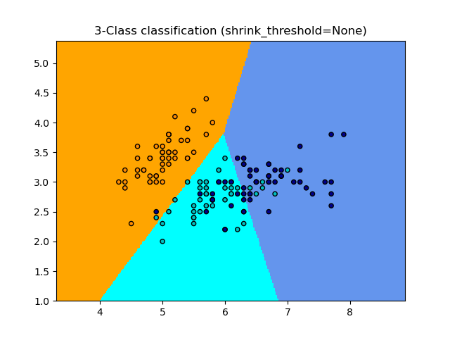
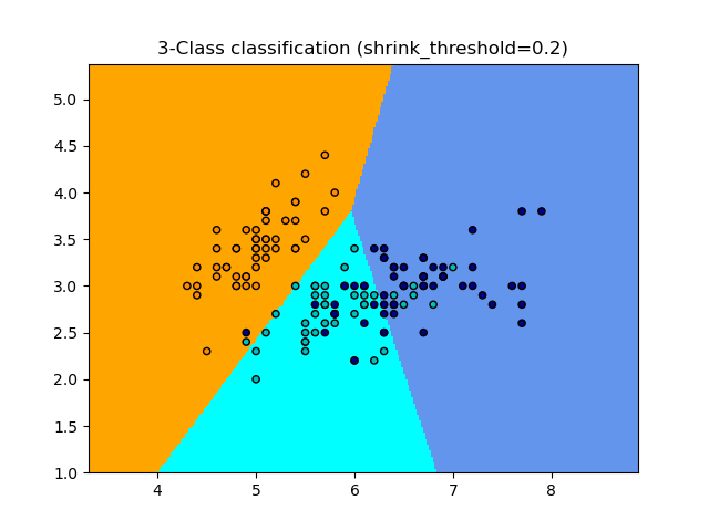
Clasificación del Centroide más Cercano

Ejemplo de uso de la clasificación del Centroide más Cercano. Trazará los límites de decisión para cada clase.

• 
• 

Out:

None 0.8133333333333334
/home/mapologo/Descargas/scikit-learn-0.24.X/examples/neighbors/plot_nearest_centroid.py:49: MatplotlibDeprecationWarning: shading='flat' when X and Y have the same dimensions as C is deprecated since 3.3.  Either specify the corners of the quadrilaterals with X and Y, or pass shading='auto', 'nearest' or 'gouraud', or set rcParams['pcolor.shading'].  This will become an error two minor releases later.
  plt.pcolormesh(xx, yy, Z, cmap=cmap_light)
0.2 0.82
/home/mapologo/Descargas/scikit-learn-0.24.X/examples/neighbors/plot_nearest_centroid.py:49: MatplotlibDeprecationWarning: shading='flat' when X and Y have the same dimensions as C is deprecated since 3.3.  Either specify the corners of the quadrilaterals with X and Y, or pass shading='auto', 'nearest' or 'gouraud', or set rcParams['pcolor.shading'].  This will become an error two minor releases later.
  plt.pcolormesh(xx, yy, Z, cmap=cmap_light)

print(__doc__)

import numpy as np
import matplotlib.pyplot as plt
from matplotlib.colors import ListedColormap
from sklearn import datasets
from sklearn.neighbors import NearestCentroid

n_neighbors = 15

# import some data to play with
iris = datasets.load_iris()
# we only take the first two features. We could avoid this ugly
# slicing by using a two-dim dataset
X = iris.data[:, :2]
y = iris.target

h = .02  # step size in the mesh

# Create color maps
cmap_light = ListedColormap(['orange', 'cyan', 'cornflowerblue'])
cmap_bold = ListedColormap(['darkorange', 'c', 'darkblue'])

for shrinkage in [None, .2]:
    # we create an instance of Neighbours Classifier and fit the data.
    clf = NearestCentroid(shrink_threshold=shrinkage)
    clf.fit(X, y)
    y_pred = clf.predict(X)
    print(shrinkage, np.mean(y == y_pred))
    # Plot the decision boundary. For that, we will assign a color to each
    # point in the mesh [x_min, x_max]x[y_min, y_max].
    x_min, x_max = X[:, 0].min() - 1, X[:, 0].max() + 1
    y_min, y_max = X[:, 1].min() - 1, X[:, 1].max() + 1
    xx, yy = np.meshgrid(np.arange(x_min, x_max, h),
                         np.arange(y_min, y_max, h))
    Z = clf.predict(np.c_[xx.ravel(), yy.ravel()])

    # Put the result into a color plot
    Z = Z.reshape(xx.shape)
    plt.figure()
    plt.pcolormesh(xx, yy, Z, cmap=cmap_light)

    # Plot also the training points
    plt.scatter(X[:, 0], X[:, 1], c=y, cmap=cmap_bold,
                edgecolor='k', s=20)
    plt.title("3-Class classification (shrink_threshold=%r)"
              % shrinkage)
    plt.axis('tight')

plt.show()