Comparación entre la búsqueda en cuadrícula y la reducción sucesiva a la mitad

Este ejemplo compara la búsqueda de parámetros realizada por HalvingGridSearchCV y GridSearchCV.

from time import time

import matplotlib.pyplot as plt
import numpy as np
import pandas as pd

from sklearn.svm import SVC
from sklearn import datasets
from sklearn.model_selection import GridSearchCV
from sklearn.experimental import enable_halving_search_cv  # noqa
from sklearn.model_selection import HalvingGridSearchCV


print(__doc__)

Primero definimos el espacio de parámetros para un estimador SVC, y calculamos el tiempo necesario para entrenar una instancia HalvingGridSearchCV, así como una instancia GridSearchCV.

rng = np.random.RandomState(0)
X, y = datasets.make_classification(n_samples=1000, random_state=rng)

gammas = [1e-1, 1e-2, 1e-3, 1e-4, 1e-5, 1e-6, 1e-7]
Cs = [1, 10, 100, 1e3, 1e4, 1e5]
param_grid = {'gamma': gammas, 'C': Cs}

clf = SVC(random_state=rng)

tic = time()
gsh = HalvingGridSearchCV(estimator=clf, param_grid=param_grid, factor=2,
                          random_state=rng)
gsh.fit(X, y)
gsh_time = time() - tic

tic = time()
gs = GridSearchCV(estimator=clf, param_grid=param_grid)
gs.fit(X, y)
gs_time = time() - tic

A continuación, graficamos los mapas de calor para ambos estimadores de búsqueda.

def make_heatmap(ax, gs, is_sh=False, make_cbar=False):
    """Helper to make a heatmap."""
    results = pd.DataFrame.from_dict(gs.cv_results_)
    results['params_str'] = results.params.apply(str)
    if is_sh:
        # SH dataframe: get mean_test_score values for the highest iter
        scores_matrix = results.sort_values('iter').pivot_table(
                index='param_gamma', columns='param_C',
                values='mean_test_score', aggfunc='last'
        )
    else:
        scores_matrix = results.pivot(index='param_gamma', columns='param_C',
                                      values='mean_test_score')

    im = ax.imshow(scores_matrix)

    ax.set_xticks(np.arange(len(Cs)))
    ax.set_xticklabels(['{:.0E}'.format(x) for x in Cs])
    ax.set_xlabel('C', fontsize=15)

    ax.set_yticks(np.arange(len(gammas)))
    ax.set_yticklabels(['{:.0E}'.format(x) for x in gammas])
    ax.set_ylabel('gamma', fontsize=15)

    # Rotate the tick labels and set their alignment.
    plt.setp(ax.get_xticklabels(), rotation=45, ha="right",
             rotation_mode="anchor")

    if is_sh:
        iterations = results.pivot_table(index='param_gamma',
                                         columns='param_C', values='iter',
                                         aggfunc='max').values
        for i in range(len(gammas)):
            for j in range(len(Cs)):
                ax.text(j, i, iterations[i, j],
                        ha="center", va="center", color="w", fontsize=20)

    if make_cbar:
        fig.subplots_adjust(right=0.8)
        cbar_ax = fig.add_axes([0.85, 0.15, 0.05, 0.7])
        fig.colorbar(im, cax=cbar_ax)
        cbar_ax.set_ylabel('mean_test_score', rotation=-90, va="bottom",
                           fontsize=15)


fig, axes = plt.subplots(ncols=2, sharey=True)
ax1, ax2 = axes

make_heatmap(ax1, gsh, is_sh=True)
make_heatmap(ax2, gs, make_cbar=True)

ax1.set_title('Successive Halving\ntime = {:.3f}s'.format(gsh_time),
              fontsize=15)
ax2.set_title('GridSearch\ntime = {:.3f}s'.format(gs_time), fontsize=15)

plt.show()

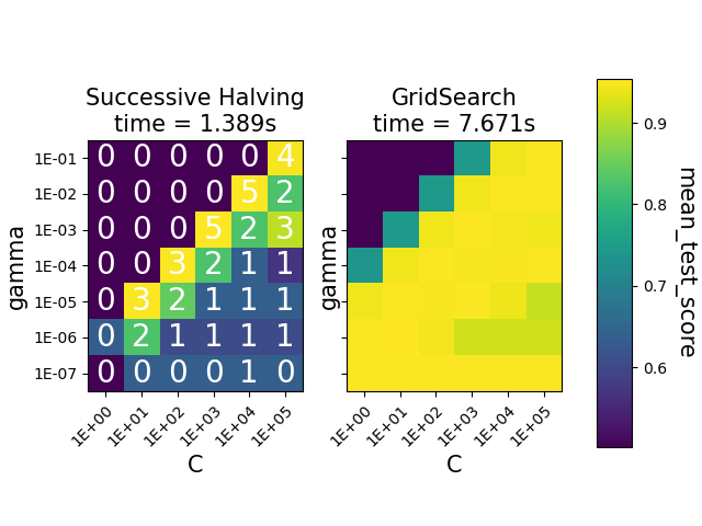
Los mapas de calor muestran la puntuación media de prueba de las combinaciones de parámetros para una instancia SVC. La HalvingGridSearchCV también muestra la iteración en la que las combinaciones fueron utilizadas por última vez. Las combinaciones marcadas como 0 sólo se evaluaron en la primera iteración, mientras que las que tienen 5 son las combinaciones de parámetros que se consideran las mejores.

Podemos ver que la clase HalvingGridSearchCV es capaz de encontrar combinaciones de parámetros tan precisas como GridSearchCV, en mucho menos tiempo.