Aprendizaje múltiple sobre dígitos manuscritos: Incrustación local lineal, Isomap…

Una ilustración de varias incrustaciones en el conjunto de datos de dígitos.

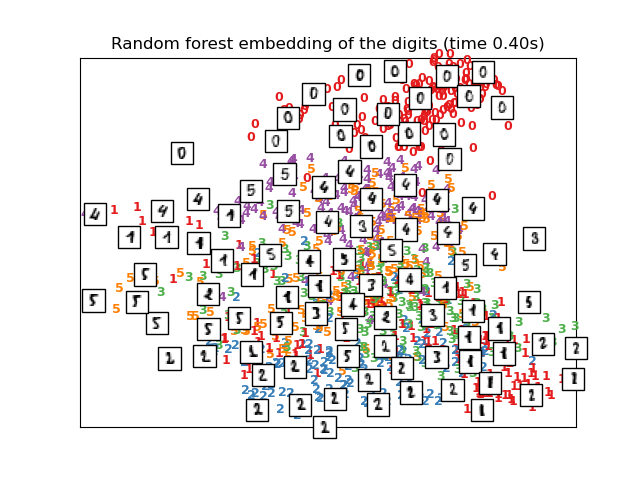
El RandomTreesEmbedding, del módulo sklearn.ensemble, no es técnicamente un método de incrustación múltiple, ya que aprende una representación de alta dimensión sobre la que aplicamos un método de reducción de la dimensionalidad. Sin embargo, a menudo es útil convertir un conjunto de datos en una representación en la que las clases son linealmente separables.

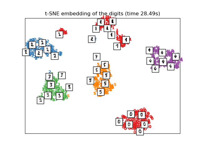
t-SNE se inicializará con la incrustación generada por PCA en este ejemplo, que no es la configuración por defecto. Garantiza la estabilidad global de la incrustación, es decir, la incrustación no depende de una inicialización aleatoria.

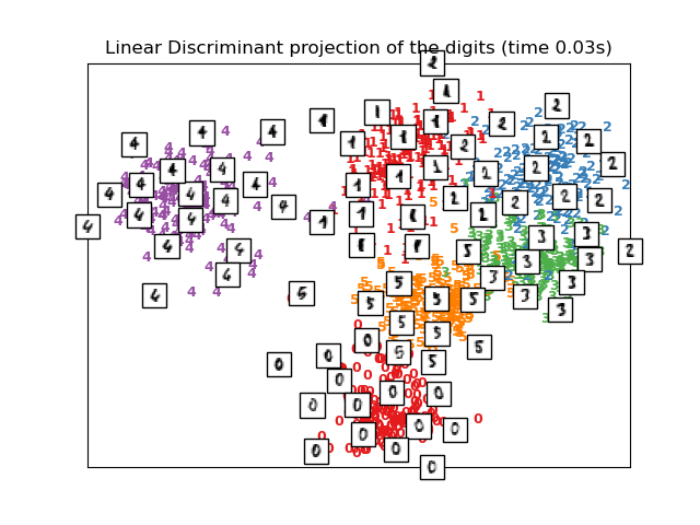
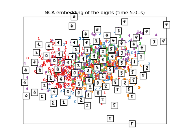
El Análisis Discriminante Lineal, del módulo sklearn.discriminant_analysis, y el Análisis de Componentes del Vecindario, del módulo sklearn.neighbors, son métodos de reducción de dimensionalidad supervisados, es decir, hacen uso de las etiquetas proporcionadas, al contrario que otros métodos.

• 
• 
• 
• 
• 
• 
• 
• 
• 
• 
• 
• 
• 
• 

Out:

Computing random projection
Computing PCA projection
Computing Linear Discriminant Analysis projection
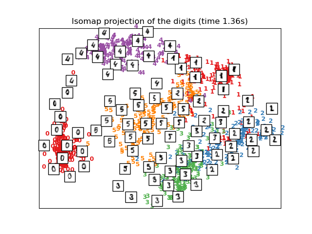
Computing Isomap projection
Done.
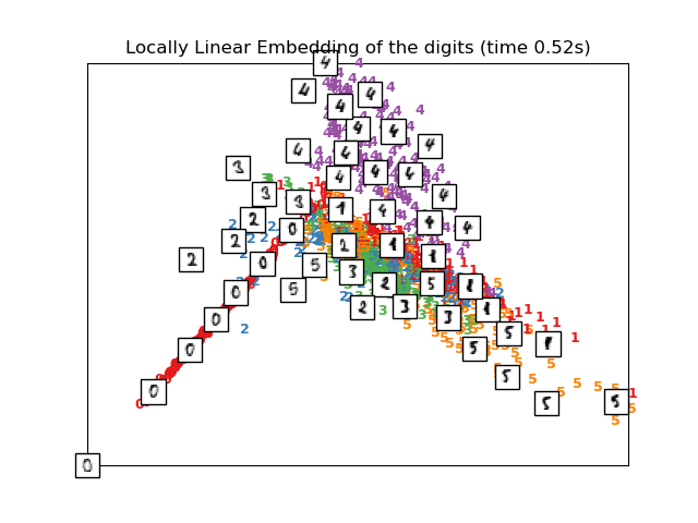
Computing LLE embedding
Done. Reconstruction error: 2.11986e-06
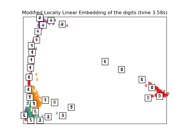
Computing modified LLE embedding
Done. Reconstruction error: 0.36082
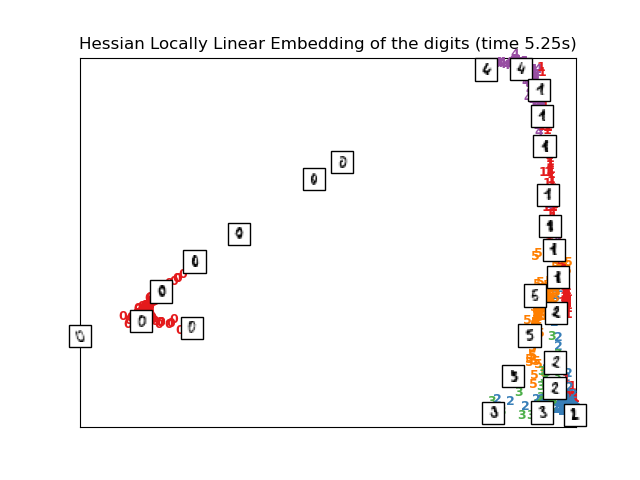
Computing Hessian LLE embedding
Done. Reconstruction error: 0.212659
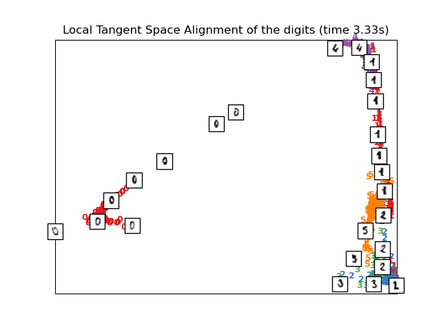
Computing LTSA embedding
Done. Reconstruction error: 0.212677
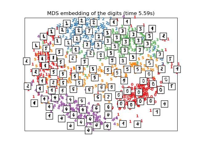
Computing MDS embedding
Done. Stress: 141386462.599449
Computing Totally Random Trees embedding
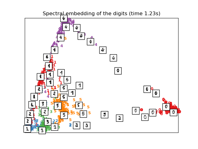
Computing Spectral embedding
Computing t-SNE embedding
Computing NCA projection

# Authors: Fabian Pedregosa <fabian.pedregosa@inria.fr>
#          Olivier Grisel <olivier.grisel@ensta.org>
#          Mathieu Blondel <mathieu@mblondel.org>
#          Gael Varoquaux
# License: BSD 3 clause (C) INRIA 2011

from time import time
import numpy as np
import matplotlib.pyplot as plt
from matplotlib import offsetbox
from sklearn import (manifold, datasets, decomposition, ensemble,
                     discriminant_analysis, random_projection, neighbors)
print(__doc__)

digits = datasets.load_digits(n_class=6)
X = digits.data
y = digits.target
n_samples, n_features = X.shape
n_neighbors = 30


# ----------------------------------------------------------------------
# Scale and visualize the embedding vectors
def plot_embedding(X, title=None):
    x_min, x_max = np.min(X, 0), np.max(X, 0)
    X = (X - x_min) / (x_max - x_min)

    plt.figure()
    ax = plt.subplot(111)
    for i in range(X.shape[0]):
        plt.text(X[i, 0], X[i, 1], str(y[i]),
                 color=plt.cm.Set1(y[i] / 10.),
                 fontdict={'weight': 'bold', 'size': 9})

    if hasattr(offsetbox, 'AnnotationBbox'):
        # only print thumbnails with matplotlib > 1.0
        shown_images = np.array([[1., 1.]])  # just something big
        for i in range(X.shape[0]):
            dist = np.sum((X[i] - shown_images) ** 2, 1)
            if np.min(dist) < 4e-3:
                # don't show points that are too close
                continue
            shown_images = np.r_[shown_images, [X[i]]]
            imagebox = offsetbox.AnnotationBbox(
                offsetbox.OffsetImage(digits.images[i], cmap=plt.cm.gray_r),
                X[i])
            ax.add_artist(imagebox)
    plt.xticks([]), plt.yticks([])
    if title is not None:
        plt.title(title)


# ----------------------------------------------------------------------
# Plot images of the digits
n_img_per_row = 20
img = np.zeros((10 * n_img_per_row, 10 * n_img_per_row))
for i in range(n_img_per_row):
    ix = 10 * i + 1
    for j in range(n_img_per_row):
        iy = 10 * j + 1
        img[ix:ix + 8, iy:iy + 8] = X[i * n_img_per_row + j].reshape((8, 8))

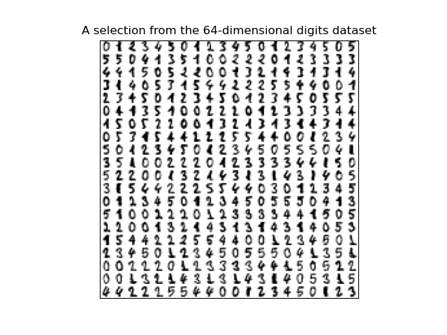
plt.imshow(img, cmap=plt.cm.binary)
plt.xticks([])
plt.yticks([])
plt.title('A selection from the 64-dimensional digits dataset')


# ----------------------------------------------------------------------
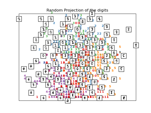
# Random 2D projection using a random unitary matrix
print("Computing random projection")
rp = random_projection.SparseRandomProjection(n_components=2, random_state=42)
X_projected = rp.fit_transform(X)
plot_embedding(X_projected, "Random Projection of the digits")


# ----------------------------------------------------------------------
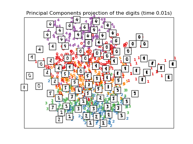
# Projection on to the first 2 principal components

print("Computing PCA projection")
t0 = time()
X_pca = decomposition.TruncatedSVD(n_components=2).fit_transform(X)
plot_embedding(X_pca,
               "Principal Components projection of the digits (time %.2fs)" %
               (time() - t0))

# ----------------------------------------------------------------------
# Projection on to the first 2 linear discriminant components

print("Computing Linear Discriminant Analysis projection")
X2 = X.copy()
X2.flat[::X.shape[1] + 1] += 0.01  # Make X invertible
t0 = time()
X_lda = discriminant_analysis.LinearDiscriminantAnalysis(n_components=2
                                                         ).fit_transform(X2, y)
plot_embedding(X_lda,
               "Linear Discriminant projection of the digits (time %.2fs)" %
               (time() - t0))


# ----------------------------------------------------------------------
# Isomap projection of the digits dataset
print("Computing Isomap projection")
t0 = time()
X_iso = manifold.Isomap(n_neighbors=n_neighbors, n_components=2
                        ).fit_transform(X)
print("Done.")
plot_embedding(X_iso,
               "Isomap projection of the digits (time %.2fs)" %
               (time() - t0))


# ----------------------------------------------------------------------
# Locally linear embedding of the digits dataset
print("Computing LLE embedding")
clf = manifold.LocallyLinearEmbedding(n_neighbors=n_neighbors, n_components=2,
                                      method='standard')
t0 = time()
X_lle = clf.fit_transform(X)
print("Done. Reconstruction error: %g" % clf.reconstruction_error_)
plot_embedding(X_lle,
               "Locally Linear Embedding of the digits (time %.2fs)" %
               (time() - t0))


# ----------------------------------------------------------------------
# Modified Locally linear embedding of the digits dataset
print("Computing modified LLE embedding")
clf = manifold.LocallyLinearEmbedding(n_neighbors=n_neighbors, n_components=2,
                                      method='modified')
t0 = time()
X_mlle = clf.fit_transform(X)
print("Done. Reconstruction error: %g" % clf.reconstruction_error_)
plot_embedding(X_mlle,
               "Modified Locally Linear Embedding of the digits (time %.2fs)" %
               (time() - t0))


# ----------------------------------------------------------------------
# HLLE embedding of the digits dataset
print("Computing Hessian LLE embedding")
clf = manifold.LocallyLinearEmbedding(n_neighbors=n_neighbors, n_components=2,
                                      method='hessian')
t0 = time()
X_hlle = clf.fit_transform(X)
print("Done. Reconstruction error: %g" % clf.reconstruction_error_)
plot_embedding(X_hlle,
               "Hessian Locally Linear Embedding of the digits (time %.2fs)" %
               (time() - t0))


# ----------------------------------------------------------------------
# LTSA embedding of the digits dataset
print("Computing LTSA embedding")
clf = manifold.LocallyLinearEmbedding(n_neighbors=n_neighbors, n_components=2,
                                      method='ltsa')
t0 = time()
X_ltsa = clf.fit_transform(X)
print("Done. Reconstruction error: %g" % clf.reconstruction_error_)
plot_embedding(X_ltsa,
               "Local Tangent Space Alignment of the digits (time %.2fs)" %
               (time() - t0))

# ----------------------------------------------------------------------
# MDS  embedding of the digits dataset
print("Computing MDS embedding")
clf = manifold.MDS(n_components=2, n_init=1, max_iter=100)
t0 = time()
X_mds = clf.fit_transform(X)
print("Done. Stress: %f" % clf.stress_)
plot_embedding(X_mds,
               "MDS embedding of the digits (time %.2fs)" %
               (time() - t0))

# ----------------------------------------------------------------------
# Random Trees embedding of the digits dataset
print("Computing Totally Random Trees embedding")
hasher = ensemble.RandomTreesEmbedding(n_estimators=200, random_state=0,
                                       max_depth=5)
t0 = time()
X_transformed = hasher.fit_transform(X)
pca = decomposition.TruncatedSVD(n_components=2)
X_reduced = pca.fit_transform(X_transformed)

plot_embedding(X_reduced,
               "Random forest embedding of the digits (time %.2fs)" %
               (time() - t0))

# ----------------------------------------------------------------------
# Spectral embedding of the digits dataset
print("Computing Spectral embedding")
embedder = manifold.SpectralEmbedding(n_components=2, random_state=0,
                                      eigen_solver="arpack")
t0 = time()
X_se = embedder.fit_transform(X)

plot_embedding(X_se,
               "Spectral embedding of the digits (time %.2fs)" %
               (time() - t0))

# ----------------------------------------------------------------------
# t-SNE embedding of the digits dataset
print("Computing t-SNE embedding")
tsne = manifold.TSNE(n_components=2, init='pca', random_state=0)
t0 = time()
X_tsne = tsne.fit_transform(X)

plot_embedding(X_tsne,
               "t-SNE embedding of the digits (time %.2fs)" %
               (time() - t0))

# ----------------------------------------------------------------------
# NCA projection of the digits dataset
print("Computing NCA projection")
nca = neighbors.NeighborhoodComponentsAnalysis(init='random',
                                               n_components=2, random_state=0)
t0 = time()
X_nca = nca.fit_transform(X, y)

plot_embedding(X_nca,
               "NCA embedding of the digits (time %.2fs)" %
               (time() - t0))

plt.show()