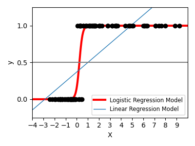
Función logística

En el gráfico se muestra cómo la regresión logística clasificaría, en este conjunto de datos sintéticos, los valores como 0 o 1, es decir, la clase uno o dos, utilizando la curva logística.

print(__doc__)


# Code source: Gael Varoquaux
# License: BSD 3 clause

import numpy as np
import matplotlib.pyplot as plt

from sklearn import linear_model
from scipy.special import expit

# General a toy dataset:s it's just a straight line with some Gaussian noise:
xmin, xmax = -5, 5
n_samples = 100
np.random.seed(0)
X = np.random.normal(size=n_samples)
y = (X > 0).astype(float)
X[X > 0] *= 4
X += .3 * np.random.normal(size=n_samples)

X = X[:, np.newaxis]

# Fit the classifier
clf = linear_model.LogisticRegression(C=1e5)
clf.fit(X, y)

# and plot the result
plt.figure(1, figsize=(4, 3))
plt.clf()
plt.scatter(X.ravel(), y, color='black', zorder=20)
X_test = np.linspace(-5, 10, 300)

loss = expit(X_test * clf.coef_ + clf.intercept_).ravel()
plt.plot(X_test, loss, color='red', linewidth=3)

ols = linear_model.LinearRegression()
ols.fit(X, y)
plt.plot(X_test, ols.coef_ * X_test + ols.intercept_, linewidth=1)
plt.axhline(.5, color='.5')

plt.ylabel('y')
plt.xlabel('X')
plt.xticks(range(-5, 10))
plt.yticks([0, 0.5, 1])
plt.ylim(-.25, 1.25)
plt.xlim(-4, 10)
plt.legend(('Logistic Regression Model', 'Linear Regression Model'),
           loc="lower right", fontsize='small')
plt.tight_layout()
plt.show()