Regresión automática de determinación de la relevancia (ARD)

Ajustar el modelo de regresión con la Regresión Bayesiana Ridge.

Consulta Regresión Bayesiana de Cresta para más información sobre el regresor.

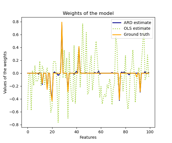
En comparación con el estimador OLS (mínimos cuadrados ordinarios), las ponderaciones de los coeficientes están ligeramente desplazadas hacia los ceros, lo que las estabiliza.

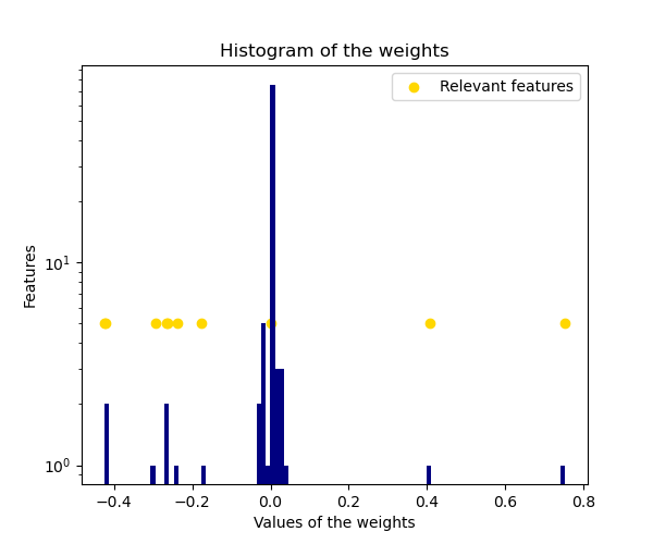
El histograma de las ponderaciones estimadas es muy puntiagudo, ya que está implícito un a priori que induce a la dispersión en las ponderaciones.

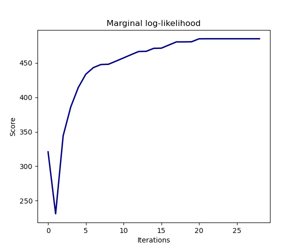
La estimación del modelo se realiza maximizando iterativamente el logaritmo de la verosimilitud marginal de las observaciones.

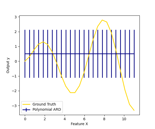
También trazamos las predicciones e incertidumbres de ARD para la regresión unidimensional utilizando la expansión de características polinómicas. Obsérvese que la incertidumbre empieza a subir en el lado derecho del gráfico. Esto se debe a que estas muestras de prueba están fuera del rango de las muestras de entrenamiento.

• 
• 
• 
• 

print(__doc__)

import numpy as np
import matplotlib.pyplot as plt
from scipy import stats

from sklearn.linear_model import ARDRegression, LinearRegression

# #############################################################################
# Generating simulated data with Gaussian weights

# Parameters of the example
np.random.seed(0)
n_samples, n_features = 100, 100
# Create Gaussian data
X = np.random.randn(n_samples, n_features)
# Create weights with a precision lambda_ of 4.
lambda_ = 4.
w = np.zeros(n_features)
# Only keep 10 weights of interest
relevant_features = np.random.randint(0, n_features, 10)
for i in relevant_features:
    w[i] = stats.norm.rvs(loc=0, scale=1. / np.sqrt(lambda_))
# Create noise with a precision alpha of 50.
alpha_ = 50.
noise = stats.norm.rvs(loc=0, scale=1. / np.sqrt(alpha_), size=n_samples)
# Create the target
y = np.dot(X, w) + noise

# #############################################################################
# Fit the ARD Regression
clf = ARDRegression(compute_score=True)
clf.fit(X, y)

ols = LinearRegression()
ols.fit(X, y)

# #############################################################################
# Plot the true weights, the estimated weights, the histogram of the
# weights, and predictions with standard deviations
plt.figure(figsize=(6, 5))
plt.title("Weights of the model")
plt.plot(clf.coef_, color='darkblue', linestyle='-', linewidth=2,
         label="ARD estimate")
plt.plot(ols.coef_, color='yellowgreen', linestyle=':', linewidth=2,
         label="OLS estimate")
plt.plot(w, color='orange', linestyle='-', linewidth=2, label="Ground truth")
plt.xlabel("Features")
plt.ylabel("Values of the weights")
plt.legend(loc=1)

plt.figure(figsize=(6, 5))
plt.title("Histogram of the weights")
plt.hist(clf.coef_, bins=n_features, color='navy', log=True)
plt.scatter(clf.coef_[relevant_features], np.full(len(relevant_features), 5.),
            color='gold', marker='o', label="Relevant features")
plt.ylabel("Features")
plt.xlabel("Values of the weights")
plt.legend(loc=1)

plt.figure(figsize=(6, 5))
plt.title("Marginal log-likelihood")
plt.plot(clf.scores_, color='navy', linewidth=2)
plt.ylabel("Score")
plt.xlabel("Iterations")


# Plotting some predictions for polynomial regression
def f(x, noise_amount):
    y = np.sqrt(x) * np.sin(x)
    noise = np.random.normal(0, 1, len(x))
    return y + noise_amount * noise


degree = 10
X = np.linspace(0, 10, 100)
y = f(X, noise_amount=1)
clf_poly = ARDRegression(threshold_lambda=1e5)
clf_poly.fit(np.vander(X, degree), y)

X_plot = np.linspace(0, 11, 25)
y_plot = f(X_plot, noise_amount=0)
y_mean, y_std = clf_poly.predict(np.vander(X_plot, degree), return_std=True)
plt.figure(figsize=(6, 5))
plt.errorbar(X_plot, y_mean, y_std, color='navy',
             label="Polynomial ARD", linewidth=2)
plt.plot(X_plot, y_plot, color='gold', linewidth=2,
         label="Ground Truth")
plt.ylabel("Output y")
plt.xlabel("Feature X")
plt.legend(loc="lower left")
plt.show()