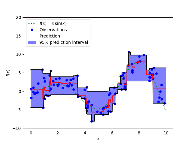
Intervalos de predicción para la Regresión con Potenciación de Gradiente

Este ejemplo muestra cómo se puede utilizar la regresión cuantílica para crear intervalos de predicción.

import numpy as np
import matplotlib.pyplot as plt

from sklearn.ensemble import GradientBoostingRegressor

np.random.seed(1)


def f(x):
    """The function to predict."""
    return x * np.sin(x)

#----------------------------------------------------------------------
#  First the noiseless case
X = np.atleast_2d(np.random.uniform(0, 10.0, size=100)).T
X = X.astype(np.float32)

# Observations
y = f(X).ravel()

dy = 1.5 + 1.0 * np.random.random(y.shape)
noise = np.random.normal(0, dy)
y += noise
y = y.astype(np.float32)

# Mesh the input space for evaluations of the real function, the prediction and
# its MSE
xx = np.atleast_2d(np.linspace(0, 10, 1000)).T
xx = xx.astype(np.float32)

alpha = 0.95

clf = GradientBoostingRegressor(loss='quantile', alpha=alpha,
                                n_estimators=250, max_depth=3,
                                learning_rate=.1, min_samples_leaf=9,
                                min_samples_split=9)

clf.fit(X, y)

# Make the prediction on the meshed x-axis
y_upper = clf.predict(xx)

clf.set_params(alpha=1.0 - alpha)
clf.fit(X, y)

# Make the prediction on the meshed x-axis
y_lower = clf.predict(xx)

clf.set_params(loss='ls')
clf.fit(X, y)

# Make the prediction on the meshed x-axis
y_pred = clf.predict(xx)

# Plot the function, the prediction and the 95% confidence interval based on
# the MSE
fig = plt.figure()
plt.plot(xx, f(xx), 'g:', label=r'$f(x) = x\,\sin(x)$')
plt.plot(X, y, 'b.', markersize=10, label=u'Observations')
plt.plot(xx, y_pred, 'r-', label=u'Prediction')
plt.plot(xx, y_upper, 'k-')
plt.plot(xx, y_lower, 'k-')
plt.fill(np.concatenate([xx, xx[::-1]]),
         np.concatenate([y_upper, y_lower[::-1]]),
         alpha=.5, fc='b', ec='None', label='95% prediction interval')
plt.xlabel('$x$')
plt.ylabel('$f(x)$')
plt.ylim(-10, 20)
plt.legend(loc='upper left')
plt.show()