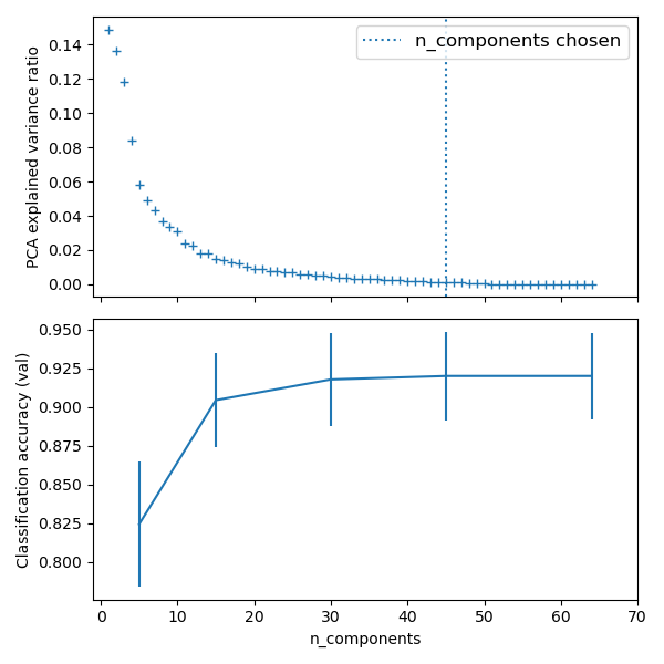
Pipelining: encadenamiento de un PCA y una regresión logística

El PCA realiza una reducción de la dimensionalidad no supervisada, mientras que la regresión logística realiza la predicción.

Utilizamos un GridSearchCV para establecer la dimensionalidad del PCA

Out:

Best parameter (CV score=0.920):
{'logistic__C': 0.046415888336127774, 'pca__n_components': 45}

print(__doc__)


# Code source: Gaël Varoquaux
# Modified for documentation by Jaques Grobler
# License: BSD 3 clause


import numpy as np
import matplotlib.pyplot as plt
import pandas as pd

from sklearn import datasets
from sklearn.decomposition import PCA
from sklearn.linear_model import LogisticRegression
from sklearn.pipeline import Pipeline
from sklearn.model_selection import GridSearchCV


# Define a pipeline to search for the best combination of PCA truncation
# and classifier regularization.
pca = PCA()
# set the tolerance to a large value to make the example faster
logistic = LogisticRegression(max_iter=10000, tol=0.1)
pipe = Pipeline(steps=[('pca', pca), ('logistic', logistic)])

X_digits, y_digits = datasets.load_digits(return_X_y=True)

# Parameters of pipelines can be set using ‘__’ separated parameter names:
param_grid = {
    'pca__n_components': [5, 15, 30, 45, 64],
    'logistic__C': np.logspace(-4, 4, 4),
}
search = GridSearchCV(pipe, param_grid, n_jobs=-1)
search.fit(X_digits, y_digits)
print("Best parameter (CV score=%0.3f):" % search.best_score_)
print(search.best_params_)

# Plot the PCA spectrum
pca.fit(X_digits)

fig, (ax0, ax1) = plt.subplots(nrows=2, sharex=True, figsize=(6, 6))
ax0.plot(np.arange(1, pca.n_components_ + 1),
         pca.explained_variance_ratio_, '+', linewidth=2)
ax0.set_ylabel('PCA explained variance ratio')

ax0.axvline(search.best_estimator_.named_steps['pca'].n_components,
            linestyle=':', label='n_components chosen')
ax0.legend(prop=dict(size=12))

# For each number of components, find the best classifier results
results = pd.DataFrame(search.cv_results_)
components_col = 'param_pca__n_components'
best_clfs = results.groupby(components_col).apply(
    lambda g: g.nlargest(1, 'mean_test_score'))

best_clfs.plot(x=components_col, y='mean_test_score', yerr='std_test_score',
               legend=False, ax=ax1)
ax1.set_ylabel('Classification accuracy (val)')
ax1.set_xlabel('n_components')

plt.xlim(-1, 70)

plt.tight_layout()
plt.show()