Parámetros RBF SVM

Este ejemplo ilustra el efecto de los parámetros gamma y C de la función de base radial (RBF) del núcleo SVM.

Intuitivamente, el parámetro gamma define hasta dónde llega la influencia de un solo ejemplo de entrenamiento, con valores bajos que significan “lejos” y valores altos que significan “cerca”. Los parámetros gamma pueden verse como la inversa del radio de influencia de las muestras seleccionadas por el modelo como vectores de soporte.

El parámetro «C» compensa la clasificación correcta de los ejemplos de entrenamiento con la maximización del margen de la función de decisión. Para valores mayores de C, se aceptará un margen menor si la función de decisión es mejor para clasificar correctamente todos los puntos de entrenamiento. Un valor más bajo de C fomentará un margen mayor y, por tanto, una función de decisión más sencilla, a costa de la precisión del entrenamiento. En otras palabras, C se comporta como un parámetro de regularización en la SVM.

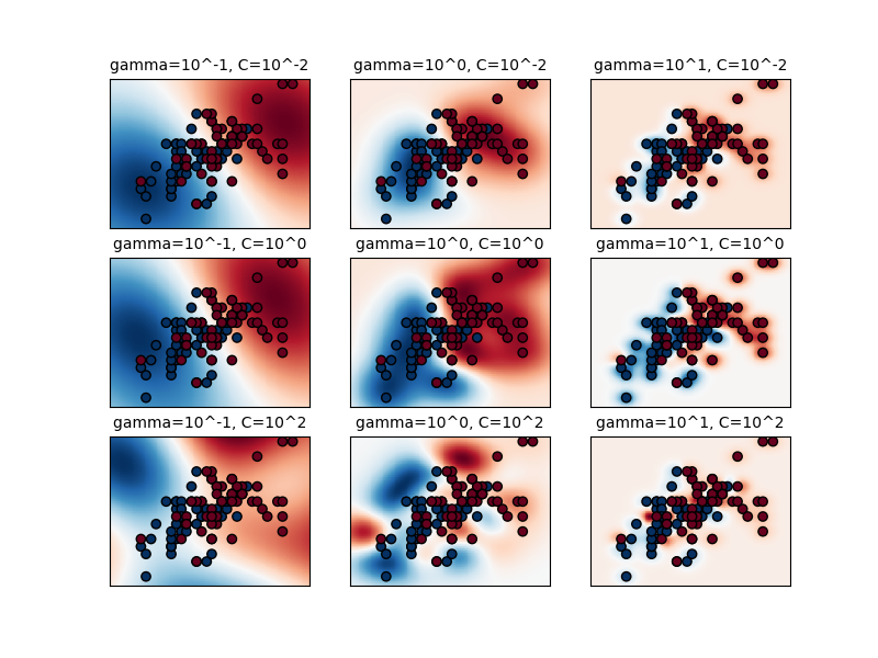
El primer gráfico es una visualización de la función de decisión para una variedad de valores de parámetros en un problema de clasificación simplificado que implica sólo 2 características de entrada y 2 posibles clases de destino (clasificación binaria). Tenga en cuenta que este tipo de gráfico no es posible para problemas con más características o clases de destino.

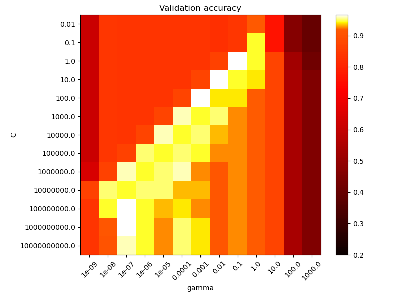
El segundo gráfico es un mapa de calor de la exactitud del clasificador de validación cruzada en función de C y gamma. Para este ejemplo, exploramos una cuadrícula relativamente grande con fines ilustrativos. En la práctica, una cuadrícula logarítmica de \(10^{-3}\) a \(10^3\) suele ser suficiente. Si los mejores parámetros se encuentran en los límites de la cuadrícula, se puede ampliar en esa dirección en una búsqueda posterior.

Ten en cuenta que la gráfica del mapa de calor tiene una barra de colores especial con un valor medio cercano a los valores de puntuación de los modelos de mejor rendimiento para que sea fácil distinguirlos en el parpadeo de un ojo.

El comportamiento del modelo es muy sensible al parámetro gamma. Si gamma es demasiado grande, el radio del área de influencia de los vectores de soporte sólo incluye el vector de soporte en sí mismo y ninguna cantidad de regularización con C será capaz de prevenir el sobrecalentamiento.

Cuando gamma es muy pequeño, el modelo es demasiado limitado y no puede capturar la complejidad o la «forma» de los datos. La región de influencia de cualquier vector de apoyo seleccionado incluiría todo el conjunto de capacitación. El modelo resultante se comportará de forma similar a un modelo lineal con un conjunto de hiperplanos que separan los centros de alta densidad de cualquier par de dos clases.

Para valores intermedios podemos ver en la segunda trama que los buenos modelos se pueden encontrar en un diagnóstico de C y gamma. Los modelos suavizados (valores inferiores de gamma) se pueden hacer más complejos aumentando la importancia de clasificar correctamente cada punto (valores más grandes C) de ahí el diagnóstico de modelos de buen rendimiento.

Por último, también se puede observar que para algunos valores intermedios de gamma se obtienen modelos de igual rendimiento cuando C se hace muy grande. Esto sugiere que el conjunto de vectores de soporte ya no cambia. El radio del núcleo RBF actúa por sí solo como un buen regularizador estructural. Aumentar C más no ayuda, probablemente porque no hay más puntos de entrenamiento en violación (dentro del margen o mal clasificados), o al menos no se puede encontrar una solución mejor. En igualdad de condiciones, puede tener sentido utilizar los valores más pequeños de C, ya que los valores muy altos de C suelen aumentar el tiempo de ajuste.

Por otro lado, los valores más bajos de C generalmente llevan a más vectores de soporte, lo que puede aumentar el tiempo de predicción. Por lo tanto, reducir el valor de C implica una compensación entre el tiempo de ajuste y el tiempo de predicción.

También debemos tener en cuenta que las pequeñas diferencias en las puntuaciones se deben a las divisiones aleatorias del procedimiento de validación cruzada. Esas variaciones espurias pueden suavizarse aumentando el número de iteraciones de CV n_splits a expensas del tiempo de cálculo. Aumentar el número de valores de los pasos C_range y gamma_range aumentará la resolución del mapa de calor de los hiperparámetros.

• 
• 

Out:

The best parameters are {'C': 1.0, 'gamma': 0.1} with a score of 0.97
/home/mapologo/Descargas/scikit-learn-0.24.X/examples/svm/plot_rbf_parameters.py:177: MatplotlibDeprecationWarning: shading='flat' when X and Y have the same dimensions as C is deprecated since 3.3.  Either specify the corners of the quadrilaterals with X and Y, or pass shading='auto', 'nearest' or 'gouraud', or set rcParams['pcolor.shading'].  This will become an error two minor releases later.
  plt.pcolormesh(xx, yy, -Z, cmap=plt.cm.RdBu)
/home/mapologo/Descargas/scikit-learn-0.24.X/examples/svm/plot_rbf_parameters.py:177: MatplotlibDeprecationWarning: shading='flat' when X and Y have the same dimensions as C is deprecated since 3.3.  Either specify the corners of the quadrilaterals with X and Y, or pass shading='auto', 'nearest' or 'gouraud', or set rcParams['pcolor.shading'].  This will become an error two minor releases later.
  plt.pcolormesh(xx, yy, -Z, cmap=plt.cm.RdBu)
/home/mapologo/Descargas/scikit-learn-0.24.X/examples/svm/plot_rbf_parameters.py:177: MatplotlibDeprecationWarning: shading='flat' when X and Y have the same dimensions as C is deprecated since 3.3.  Either specify the corners of the quadrilaterals with X and Y, or pass shading='auto', 'nearest' or 'gouraud', or set rcParams['pcolor.shading'].  This will become an error two minor releases later.
  plt.pcolormesh(xx, yy, -Z, cmap=plt.cm.RdBu)
/home/mapologo/Descargas/scikit-learn-0.24.X/examples/svm/plot_rbf_parameters.py:177: MatplotlibDeprecationWarning: shading='flat' when X and Y have the same dimensions as C is deprecated since 3.3.  Either specify the corners of the quadrilaterals with X and Y, or pass shading='auto', 'nearest' or 'gouraud', or set rcParams['pcolor.shading'].  This will become an error two minor releases later.
  plt.pcolormesh(xx, yy, -Z, cmap=plt.cm.RdBu)
/home/mapologo/Descargas/scikit-learn-0.24.X/examples/svm/plot_rbf_parameters.py:177: MatplotlibDeprecationWarning: shading='flat' when X and Y have the same dimensions as C is deprecated since 3.3.  Either specify the corners of the quadrilaterals with X and Y, or pass shading='auto', 'nearest' or 'gouraud', or set rcParams['pcolor.shading'].  This will become an error two minor releases later.
  plt.pcolormesh(xx, yy, -Z, cmap=plt.cm.RdBu)
/home/mapologo/Descargas/scikit-learn-0.24.X/examples/svm/plot_rbf_parameters.py:177: MatplotlibDeprecationWarning: shading='flat' when X and Y have the same dimensions as C is deprecated since 3.3.  Either specify the corners of the quadrilaterals with X and Y, or pass shading='auto', 'nearest' or 'gouraud', or set rcParams['pcolor.shading'].  This will become an error two minor releases later.
  plt.pcolormesh(xx, yy, -Z, cmap=plt.cm.RdBu)
/home/mapologo/Descargas/scikit-learn-0.24.X/examples/svm/plot_rbf_parameters.py:177: MatplotlibDeprecationWarning: shading='flat' when X and Y have the same dimensions as C is deprecated since 3.3.  Either specify the corners of the quadrilaterals with X and Y, or pass shading='auto', 'nearest' or 'gouraud', or set rcParams['pcolor.shading'].  This will become an error two minor releases later.
  plt.pcolormesh(xx, yy, -Z, cmap=plt.cm.RdBu)
/home/mapologo/Descargas/scikit-learn-0.24.X/examples/svm/plot_rbf_parameters.py:177: MatplotlibDeprecationWarning: shading='flat' when X and Y have the same dimensions as C is deprecated since 3.3.  Either specify the corners of the quadrilaterals with X and Y, or pass shading='auto', 'nearest' or 'gouraud', or set rcParams['pcolor.shading'].  This will become an error two minor releases later.
  plt.pcolormesh(xx, yy, -Z, cmap=plt.cm.RdBu)
/home/mapologo/Descargas/scikit-learn-0.24.X/examples/svm/plot_rbf_parameters.py:177: MatplotlibDeprecationWarning: shading='flat' when X and Y have the same dimensions as C is deprecated since 3.3.  Either specify the corners of the quadrilaterals with X and Y, or pass shading='auto', 'nearest' or 'gouraud', or set rcParams['pcolor.shading'].  This will become an error two minor releases later.
  plt.pcolormesh(xx, yy, -Z, cmap=plt.cm.RdBu)

print(__doc__)

import numpy as np
import matplotlib.pyplot as plt
from matplotlib.colors import Normalize

from sklearn.svm import SVC
from sklearn.preprocessing import StandardScaler
from sklearn.datasets import load_iris
from sklearn.model_selection import StratifiedShuffleSplit
from sklearn.model_selection import GridSearchCV


# Utility function to move the midpoint of a colormap to be around
# the values of interest.

class MidpointNormalize(Normalize):

    def __init__(self, vmin=None, vmax=None, midpoint=None, clip=False):
        self.midpoint = midpoint
        Normalize.__init__(self, vmin, vmax, clip)

    def __call__(self, value, clip=None):
        x, y = [self.vmin, self.midpoint, self.vmax], [0, 0.5, 1]
        return np.ma.masked_array(np.interp(value, x, y))

# #############################################################################
# Load and prepare data set
#
# dataset for grid search

iris = load_iris()
X = iris.data
y = iris.target

# Dataset for decision function visualization: we only keep the first two
# features in X and sub-sample the dataset to keep only 2 classes and
# make it a binary classification problem.

X_2d = X[:, :2]
X_2d = X_2d[y > 0]
y_2d = y[y > 0]
y_2d -= 1

# It is usually a good idea to scale the data for SVM training.
# We are cheating a bit in this example in scaling all of the data,
# instead of fitting the transformation on the training set and
# just applying it on the test set.

scaler = StandardScaler()
X = scaler.fit_transform(X)
X_2d = scaler.fit_transform(X_2d)

# #############################################################################
# Train classifiers
#
# For an initial search, a logarithmic grid with basis
# 10 is often helpful. Using a basis of 2, a finer
# tuning can be achieved but at a much higher cost.

C_range = np.logspace(-2, 10, 13)
gamma_range = np.logspace(-9, 3, 13)
param_grid = dict(gamma=gamma_range, C=C_range)
cv = StratifiedShuffleSplit(n_splits=5, test_size=0.2, random_state=42)
grid = GridSearchCV(SVC(), param_grid=param_grid, cv=cv)
grid.fit(X, y)

print("The best parameters are %s with a score of %0.2f"
      % (grid.best_params_, grid.best_score_))

# Now we need to fit a classifier for all parameters in the 2d version
# (we use a smaller set of parameters here because it takes a while to train)

C_2d_range = [1e-2, 1, 1e2]
gamma_2d_range = [1e-1, 1, 1e1]
classifiers = []
for C in C_2d_range:
    for gamma in gamma_2d_range:
        clf = SVC(C=C, gamma=gamma)
        clf.fit(X_2d, y_2d)
        classifiers.append((C, gamma, clf))

# #############################################################################
# Visualization
#
# draw visualization of parameter effects

plt.figure(figsize=(8, 6))
xx, yy = np.meshgrid(np.linspace(-3, 3, 200), np.linspace(-3, 3, 200))
for (k, (C, gamma, clf)) in enumerate(classifiers):
    # evaluate decision function in a grid
    Z = clf.decision_function(np.c_[xx.ravel(), yy.ravel()])
    Z = Z.reshape(xx.shape)

    # visualize decision function for these parameters
    plt.subplot(len(C_2d_range), len(gamma_2d_range), k + 1)
    plt.title("gamma=10^%d, C=10^%d" % (np.log10(gamma), np.log10(C)),
              size='medium')

    # visualize parameter's effect on decision function
    plt.pcolormesh(xx, yy, -Z, cmap=plt.cm.RdBu)
    plt.scatter(X_2d[:, 0], X_2d[:, 1], c=y_2d, cmap=plt.cm.RdBu_r,
                edgecolors='k')
    plt.xticks(())
    plt.yticks(())
    plt.axis('tight')

scores = grid.cv_results_['mean_test_score'].reshape(len(C_range),
                                                     len(gamma_range))

# Draw heatmap of the validation accuracy as a function of gamma and C
#
# The score are encoded as colors with the hot colormap which varies from dark
# red to bright yellow. As the most interesting scores are all located in the
# 0.92 to 0.97 range we use a custom normalizer to set the mid-point to 0.92 so
# as to make it easier to visualize the small variations of score values in the
# interesting range while not brutally collapsing all the low score values to
# the same color.

plt.figure(figsize=(8, 6))
plt.subplots_adjust(left=.2, right=0.95, bottom=0.15, top=0.95)
plt.imshow(scores, interpolation='nearest', cmap=plt.cm.hot,
           norm=MidpointNormalize(vmin=0.2, midpoint=0.92))
plt.xlabel('gamma')
plt.ylabel('C')
plt.colorbar()
plt.xticks(np.arange(len(gamma_range)), gamma_range, rotation=45)
plt.yticks(np.arange(len(C_range)), C_range)
plt.title('Validation accuracy')
plt.show()