Dígitos de Propagación de Etiquetas: Demostración del rendimiento

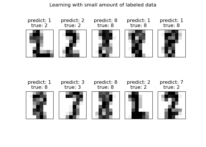
Este ejemplo demuestra la potencia del aprendizaje semisupervisado al entrenar un modelo de Propagación de Etiquetas (Label Spreading model) para clasificar dígitos escritos a mano con conjuntos de muy pocas etiquetas.

El conjunto de datos de dígitos escritos a mano tiene 1797 puntos en total. El modelo se entrenará utilizando todos los puntos, pero sólo se etiquetarán 30. Los resultados en forma de una matriz de confusión y una serie de métricas sobre cada clase serán muy buenos.

Al final, se mostrarán las 10 predicciones más inciertas.

Out:

Label Spreading model: 40 labeled & 300 unlabeled points (340 total)
              precision    recall  f1-score   support

           0       1.00      1.00      1.00        27
           1       0.82      1.00      0.90        37
           2       1.00      0.86      0.92        28
           3       1.00      0.80      0.89        35
           4       0.92      1.00      0.96        24
           5       0.74      0.94      0.83        34
           6       0.89      0.96      0.92        25
           7       0.94      0.89      0.91        35
           8       1.00      0.68      0.81        31
           9       0.81      0.88      0.84        24

    accuracy                           0.90       300
   macro avg       0.91      0.90      0.90       300
weighted avg       0.91      0.90      0.90       300

Confusion matrix
[[27  0  0  0  0  0  0  0  0  0]
 [ 0 37  0  0  0  0  0  0  0  0]
 [ 0  1 24  0  0  0  2  1  0  0]
 [ 0  0  0 28  0  5  0  1  0  1]
 [ 0  0  0  0 24  0  0  0  0  0]
 [ 0  0  0  0  0 32  0  0  0  2]
 [ 0  0  0  0  0  1 24  0  0  0]
 [ 0  0  0  0  1  3  0 31  0  0]
 [ 0  7  0  0  0  0  1  0 21  2]
 [ 0  0  0  0  1  2  0  0  0 21]]

print(__doc__)

# Authors: Clay Woolam <clay@woolam.org>
# License: BSD

import numpy as np
import matplotlib.pyplot as plt

from scipy import stats

from sklearn import datasets
from sklearn.semi_supervised import LabelSpreading

from sklearn.metrics import confusion_matrix, classification_report

digits = datasets.load_digits()
rng = np.random.RandomState(2)
indices = np.arange(len(digits.data))
rng.shuffle(indices)

X = digits.data[indices[:340]]
y = digits.target[indices[:340]]
images = digits.images[indices[:340]]

n_total_samples = len(y)
n_labeled_points = 40

indices = np.arange(n_total_samples)

unlabeled_set = indices[n_labeled_points:]

# #############################################################################
# Shuffle everything around
y_train = np.copy(y)
y_train[unlabeled_set] = -1

# #############################################################################
# Learn with LabelSpreading
lp_model = LabelSpreading(gamma=.25, max_iter=20)
lp_model.fit(X, y_train)
predicted_labels = lp_model.transduction_[unlabeled_set]
true_labels = y[unlabeled_set]

cm = confusion_matrix(true_labels, predicted_labels, labels=lp_model.classes_)

print("Label Spreading model: %d labeled & %d unlabeled points (%d total)" %
      (n_labeled_points, n_total_samples - n_labeled_points, n_total_samples))

print(classification_report(true_labels, predicted_labels))

print("Confusion matrix")
print(cm)

# #############################################################################
# Calculate uncertainty values for each transduced distribution
pred_entropies = stats.distributions.entropy(lp_model.label_distributions_.T)

# #############################################################################
# Pick the top 10 most uncertain labels
uncertainty_index = np.argsort(pred_entropies)[-10:]

# #############################################################################
# Plot
f = plt.figure(figsize=(7, 5))
for index, image_index in enumerate(uncertainty_index):
    image = images[image_index]

    sub = f.add_subplot(2, 5, index + 1)
    sub.imshow(image, cmap=plt.cm.gray_r)
    plt.xticks([])
    plt.yticks([])
    sub.set_title('predict: %i\ntrue: %i' % (
        lp_model.transduction_[image_index], y[image_index]))

f.suptitle('Learning with small amount of labeled data')
plt.show()