Características de la Máquina de Boltzmann restringida para la clasificación de dígitos

Para los datos de imágenes en escala de grises en los que los valores de los píxeles pueden interpretarse como grados de negrura sobre un fondo blanco, como el reconocimiento de dígitos escritos a mano, el modelo de la máquina de Boltzmann restringida Bernoulli (BernoulliRBM) puede realizar una eficaz extracción de características no lineales.

Para aprender buenas representaciones latentes a partir de un conjunto de datos pequeño, generamos artificialmente más datos etiquetados perturbando los datos de entrenamiento con desplazamientos lineales de 1 píxel en cada dirección.

Este ejemplo muestra cómo construir un pipeline de clasificación con un extractor de características BernoulliRBM y un clasificador LogisticRegression. Los hiperparámetros de todo el modelo (tasa de aprendizaje, tamaño de la capa oculta, regularización) se optimizaron mediante la búsqueda en cuadrícula, pero la búsqueda no se reproduce aquí debido a las restricciones de tiempo de ejecución.

A modo de comparación, se presenta una regresión logística sobre los valores en bruto de los píxeles. El ejemplo muestra que las características extraídas por la BernoulliRBM ayudan a mejorar la exactitud de la clasificación.

Out:

[BernoulliRBM] Iteration 1, pseudo-likelihood = -25.39, time = 0.16s
[BernoulliRBM] Iteration 2, pseudo-likelihood = -23.77, time = 0.28s
[BernoulliRBM] Iteration 3, pseudo-likelihood = -22.94, time = 0.29s
[BernoulliRBM] Iteration 4, pseudo-likelihood = -21.87, time = 0.29s
[BernoulliRBM] Iteration 5, pseudo-likelihood = -21.69, time = 0.28s
[BernoulliRBM] Iteration 6, pseudo-likelihood = -20.85, time = 0.27s
[BernoulliRBM] Iteration 7, pseudo-likelihood = -20.83, time = 0.28s
[BernoulliRBM] Iteration 8, pseudo-likelihood = -20.60, time = 0.27s
[BernoulliRBM] Iteration 9, pseudo-likelihood = -20.36, time = 0.27s
[BernoulliRBM] Iteration 10, pseudo-likelihood = -20.22, time = 0.28s
Logistic regression using RBM features:
              precision    recall  f1-score   support

           0       1.00      0.98      0.99       174
           1       0.92      0.92      0.92       184
           2       0.93      0.95      0.94       166
           3       0.95      0.87      0.91       194
           4       0.97      0.95      0.96       186
           5       0.94      0.91      0.92       181
           6       0.98      0.98      0.98       207
           7       0.94      0.99      0.96       154
           8       0.89      0.91      0.90       182
           9       0.85      0.91      0.88       169

    accuracy                           0.94      1797
   macro avg       0.94      0.94      0.94      1797
weighted avg       0.94      0.94      0.94      1797


Logistic regression using raw pixel features:
              precision    recall  f1-score   support

           0       0.90      0.91      0.91       174
           1       0.60      0.58      0.59       184
           2       0.75      0.85      0.80       166
           3       0.78      0.78      0.78       194
           4       0.81      0.83      0.82       186
           5       0.75      0.76      0.75       181
           6       0.90      0.87      0.89       207
           7       0.85      0.88      0.87       154
           8       0.67      0.59      0.63       182
           9       0.75      0.76      0.76       169

    accuracy                           0.78      1797
   macro avg       0.78      0.78      0.78      1797
weighted avg       0.78      0.78      0.78      1797

print(__doc__)

# Authors: Yann N. Dauphin, Vlad Niculae, Gabriel Synnaeve
# License: BSD

import numpy as np
import matplotlib.pyplot as plt

from scipy.ndimage import convolve
from sklearn import linear_model, datasets, metrics
from sklearn.model_selection import train_test_split
from sklearn.neural_network import BernoulliRBM
from sklearn.pipeline import Pipeline
from sklearn.base import clone


# #############################################################################
# Setting up

def nudge_dataset(X, Y):
    """
    This produces a dataset 5 times bigger than the original one,
    by moving the 8x8 images in X around by 1px to left, right, down, up
    """
    direction_vectors = [
        [[0, 1, 0],
         [0, 0, 0],
         [0, 0, 0]],

        [[0, 0, 0],
         [1, 0, 0],
         [0, 0, 0]],

        [[0, 0, 0],
         [0, 0, 1],
         [0, 0, 0]],

        [[0, 0, 0],
         [0, 0, 0],
         [0, 1, 0]]]

    def shift(x, w):
        return convolve(x.reshape((8, 8)), mode='constant', weights=w).ravel()

    X = np.concatenate([X] +
                       [np.apply_along_axis(shift, 1, X, vector)
                        for vector in direction_vectors])
    Y = np.concatenate([Y for _ in range(5)], axis=0)
    return X, Y


# Load Data
X, y = datasets.load_digits(return_X_y=True)
X = np.asarray(X, 'float32')
X, Y = nudge_dataset(X, y)
X = (X - np.min(X, 0)) / (np.max(X, 0) + 0.0001)  # 0-1 scaling

X_train, X_test, Y_train, Y_test = train_test_split(
    X, Y, test_size=0.2, random_state=0)

# Models we will use
logistic = linear_model.LogisticRegression(solver='newton-cg', tol=1)
rbm = BernoulliRBM(random_state=0, verbose=True)

rbm_features_classifier = Pipeline(
    steps=[('rbm', rbm), ('logistic', logistic)])

# #############################################################################
# Training

# Hyper-parameters. These were set by cross-validation,
# using a GridSearchCV. Here we are not performing cross-validation to
# save time.
rbm.learning_rate = 0.06
rbm.n_iter = 10
# More components tend to give better prediction performance, but larger
# fitting time
rbm.n_components = 100
logistic.C = 6000

# Training RBM-Logistic Pipeline
rbm_features_classifier.fit(X_train, Y_train)

# Training the Logistic regression classifier directly on the pixel
raw_pixel_classifier = clone(logistic)
raw_pixel_classifier.C = 100.
raw_pixel_classifier.fit(X_train, Y_train)

# #############################################################################
# Evaluation

Y_pred = rbm_features_classifier.predict(X_test)
print("Logistic regression using RBM features:\n%s\n" % (
    metrics.classification_report(Y_test, Y_pred)))

Y_pred = raw_pixel_classifier.predict(X_test)
print("Logistic regression using raw pixel features:\n%s\n" % (
    metrics.classification_report(Y_test, Y_pred)))

# #############################################################################
# Plotting

plt.figure(figsize=(4.2, 4))
for i, comp in enumerate(rbm.components_):
    plt.subplot(10, 10, i + 1)
    plt.imshow(comp.reshape((8, 8)), cmap=plt.cm.gray_r,
               interpolation='nearest')
    plt.xticks(())
    plt.yticks(())
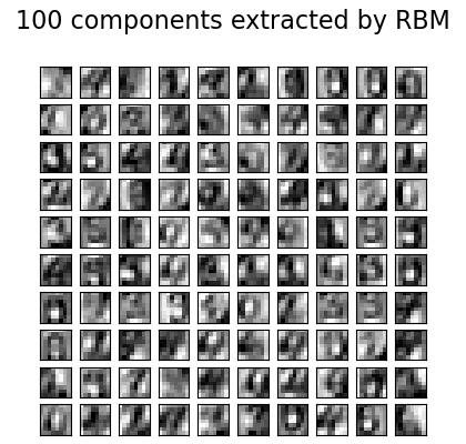
plt.suptitle('100 components extracted by RBM', fontsize=16)
plt.subplots_adjust(0.08, 0.02, 0.92, 0.85, 0.08, 0.23)

plt.show()