Comparación de Vecinos más Cercanos con y sin Análisis de Componentes del Vecindario

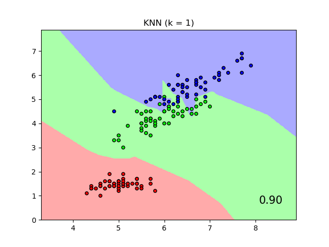
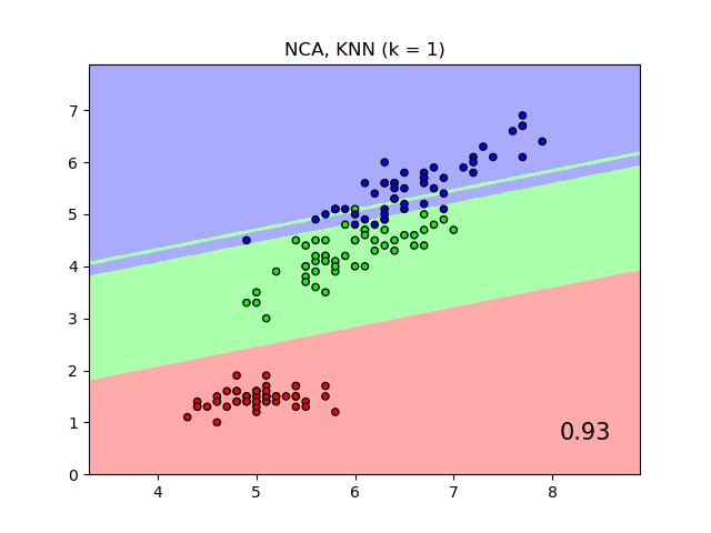
Un ejemplo que compara la clasificación de los vecinos más cercanos con y sin Análisis de Componentes del Vecindario.

Graficará los límites de decisión de clase dados por un clasificador de Vecinos más Cercanos cuando se utiliza la distancia euclidiana en las características originales, en comparación con el uso de la distancia euclidiana después de la transformación aprendida por el Análisis de Componentes del Vecindario. El objetivo de este último es encontrar una transformación lineal que maximice la precisión de la clasificación (estocástica) del vecino más cercano en el conjunto de entrenamiento.

• 
• 

Out:

/home/mapologo/Descargas/scikit-learn-0.24.X/examples/neighbors/plot_nca_classification.py:78: MatplotlibDeprecationWarning: shading='flat' when X and Y have the same dimensions as C is deprecated since 3.3.  Either specify the corners of the quadrilaterals with X and Y, or pass shading='auto', 'nearest' or 'gouraud', or set rcParams['pcolor.shading'].  This will become an error two minor releases later.
  plt.pcolormesh(xx, yy, Z, cmap=cmap_light, alpha=.8)
/home/mapologo/Descargas/scikit-learn-0.24.X/examples/neighbors/plot_nca_classification.py:78: MatplotlibDeprecationWarning: shading='flat' when X and Y have the same dimensions as C is deprecated since 3.3.  Either specify the corners of the quadrilaterals with X and Y, or pass shading='auto', 'nearest' or 'gouraud', or set rcParams['pcolor.shading'].  This will become an error two minor releases later.
  plt.pcolormesh(xx, yy, Z, cmap=cmap_light, alpha=.8)

# License: BSD 3 clause

import numpy as np
import matplotlib.pyplot as plt
from matplotlib.colors import ListedColormap
from sklearn import datasets
from sklearn.model_selection import train_test_split
from sklearn.preprocessing import StandardScaler
from sklearn.neighbors import (KNeighborsClassifier,
                               NeighborhoodComponentsAnalysis)
from sklearn.pipeline import Pipeline


print(__doc__)

n_neighbors = 1

dataset = datasets.load_iris()
X, y = dataset.data, dataset.target

# we only take two features. We could avoid this ugly
# slicing by using a two-dim dataset
X = X[:, [0, 2]]

X_train, X_test, y_train, y_test = \
    train_test_split(X, y, stratify=y, test_size=0.7, random_state=42)

h = .01  # step size in the mesh

# Create color maps
cmap_light = ListedColormap(['#FFAAAA', '#AAFFAA', '#AAAAFF'])
cmap_bold = ListedColormap(['#FF0000', '#00FF00', '#0000FF'])

names = ['KNN', 'NCA, KNN']

classifiers = [Pipeline([('scaler', StandardScaler()),
                         ('knn', KNeighborsClassifier(n_neighbors=n_neighbors))
                         ]),
               Pipeline([('scaler', StandardScaler()),
                         ('nca', NeighborhoodComponentsAnalysis()),
                         ('knn', KNeighborsClassifier(n_neighbors=n_neighbors))
                         ])
               ]

x_min, x_max = X[:, 0].min() - 1, X[:, 0].max() + 1
y_min, y_max = X[:, 1].min() - 1, X[:, 1].max() + 1
xx, yy = np.meshgrid(np.arange(x_min, x_max, h),
                     np.arange(y_min, y_max, h))

for name, clf in zip(names, classifiers):

    clf.fit(X_train, y_train)
    score = clf.score(X_test, y_test)

    # Plot the decision boundary. For that, we will assign a color to each
    # point in the mesh [x_min, x_max]x[y_min, y_max].
    Z = clf.predict(np.c_[xx.ravel(), yy.ravel()])

    # Put the result into a color plot
    Z = Z.reshape(xx.shape)
    plt.figure()
    plt.pcolormesh(xx, yy, Z, cmap=cmap_light, alpha=.8)

    # Plot also the training and testing points
    plt.scatter(X[:, 0], X[:, 1], c=y, cmap=cmap_bold, edgecolor='k', s=20)
    plt.xlim(xx.min(), xx.max())
    plt.ylim(yy.min(), yy.max())
    plt.title("{} (k = {})".format(name, n_neighbors))
    plt.text(0.9, 0.1, '{:.2f}'.format(score), size=15,
             ha='center', va='center', transform=plt.gca().transAxes)

plt.show()